Encoding in Machine Learning: Designing Categorical Geometry
A geometric and statistical exploration of encoder families — from categorical mappings to latent spaces, positional signals, and semantic retrieval encoders
Introduction
Before a model learns, before a loss is minimized, before a gradient flows, a quieter decision is made.
How do we represent the world?
A categorical variable looks innocent. A column of regions. Product IDs. User segments. Device types. We call them “features” as if they were naturally numeric, as if the model were merely waiting for them to be formatted correctly.
But a category is not a number — it is a partition, a declaration that some observations are equivalent under a certain abstraction.
The moment we transform it, we decide something far more consequential than formatting. We decide whether two categories are neighbors or strangers, whether they lie on a line or float in orthogonal isolation, whether similarity is imposed or allowed to emerge. And once we decide, the model never questions that choice.
What is distance between “France” and “Germany”? Should “Premium” be twice “Standard”? When we collapse identity into expectation, are we modeling behavior — or leaking it?
To encode — from Latin in- (“into”) and codex (“a book of rules”) — is to inscribe something into a system. In machine learning, it is the transformation of information into numerical form so a model can process it. Encoding is the first act of modeling — where epistemology becomes geometry.
1. A Taxonomy of Encoder Families
Encoding is not one technique. It is a family of techniques, each answering a different question about what structure to impose and from where.
| Family | What it encodes | Geometry imposed | Typical domain |
|---|---|---|---|
| Categorical | discrete identity | scalar or orthogonal basis | tabular ML |
| Latent Space | compressed structure | learned manifold | generative models |
| Positional | sequence order | frequency-based or learned offsets | Transformers, LLMs |
| Semantic | meaning of objects or pairs | dense vector or scalar score | NLP, retrieval |
The choice of encoder family is not a preprocessing detail — it defines what the model is allowed to know about the world.
2. Categorical Encoders
Categorical encoders address the most classical problem: a finite set of labels — regions, product types, user segments — must become numbers that a model can compute with. The mapping $f : \mathcal{C} \rightarrow \mathbb{R}^k$ looks innocent, but the choice of $f$ determines which categories appear close, which appear far, and which appear identical. Once applied, the model interacts only with the induced geometry — never again with the original labels.
| Encoder | Geometric form | Key assumption |
|---|---|---|
| Label | 1D ordered axis | Total ordering exists |
| One-Hot | Orthogonal basis | Categories fully independent |
| Ordinal | Ordered scalar | Uniform rank spacing |
| Target | Conditional mean | Outcome tendency defines identity |
| Frequency | Density scalar | Prevalence is predictive |
2.1 Label Encoding
The simplest approach: assign each category an integer. North → 0, South → 1, East → 2, and so on. The encoding is a lookup table — deterministic, no parameters.
The problem is that integers carry geometry. The model reads the distance between two values as meaningful, so North (0) and South (1) appear closer than North (0) and West (3) — purely because of the arbitrary assignment made before training began. Two different assignments for the same five regions produce different tree splits at the same threshold:
| Region | Encoding A | Encoding B |
|---|---|---|
| North | 0 | 3 |
| South | 1 | 0 |
| East | 2 | 1 |
| West | 3 | 4 |
| Central | 4 | 2 |
- Split A (
f(c) ≤ 1): {North, South} vs {East, West, Central} - Split B (
f(c) ≤ 1): {South, East} vs {North, West, Central}
Same model, same threshold — different partitions, determined solely by a choice made before training. Label encoding introduces no estimation variance (it is fully deterministic), but it injects maximal structural bias: the model is forced to treat an invented ordering as real signal.
2.2 One-Hot Encoding
One-hot encoding assigns each category its own binary column. A category is represented by a 1 in its column and 0 everywhere else — every category gets exactly one “active” dimension.
With 3 countries, the representation is clean and readable:
| Observation | is_France | is_Germany | is_UK |
|---|---|---|---|
| obs_1 | 1 | 0 | 0 |
| obs_2 | 0 | 1 | 0 |
| obs_3 | 0 | 0 | 1 |
Each observation is a point on a different axis. No category is numerically closer to another — France and Germany are exactly as far apart as France and UK. This is one-hot’s core strength: it imposes no ordering and no artificial proximity.
The geometry breaks down at scale. With 6 countries already every row is mostly zeros:
| Observation | is_FR | is_DE | is_UK | is_ES | is_IT | is_PL |
|---|---|---|---|---|---|---|
| obs_1 | 1 | 0 | 0 | 0 | 0 | 0 |
| obs_2 | 0 | 0 | 0 | 0 | 1 | 0 |
| obs_3 | 0 | 0 | 0 | 1 | 0 | 0 |
With 500 product IDs, each row is 499 zeros and 1 one. The model now has one parameter per category — and for a product that appears 3 times in training data, that parameter is estimated from those 3 observations alone. Rare categories carry high estimation variance. Memory scales with $n \times k$, and one column must be dropped when an intercept is present to avoid a perfectly collinear design matrix.
The structural bias of one-hot is near zero — no ordering is imposed, all categories are equidistant. But that structural neutrality comes at the cost of statistical variance: the sparser the data per category, the noisier the learned coefficients.
2.3 Target Encoding
Instead of encoding what a category is, target encoding encodes what it predicts. Each category is replaced by the average outcome among observations that belong to it:
\[c \mapsto \mathbb{E}[Y \mid C = c]\]A product category “Electronics” doesn’t get an integer or a binary column — it gets a number like 0.73, reflecting the mean conversion rate of that category in the training data. Two categories with similar outcome tendencies land near each other in the encoding, regardless of their names or frequencies.
When a category appears rarely, its sample average is unstable. Shrinkage pulls it toward the global mean to reduce noise:
\[\hat{\mu}_c = \frac{n_c \mu_c + \alpha \mu}{n_c + \alpha}\]With small $n_c$, the global mean $\mu$ dominates; as $n_c$ grows, the category’s own mean takes over. This makes the bias-variance tradeoff explicit: higher $\alpha$ adds bias (estimates are pulled toward the global average) but cuts variance for sparse categories.
Target leakage — if the average is computed over the full training set, each observation’s outcome contributes to its own encoding. The model sees the target baked into the feature before training.
The two tables below show how the numbers shift depending on whether the encoding is computed naïvely or out-of-fold:
Naïve (leaky): each observation contributes to its own $\hat{\mu}_c$.
| obs | category | y | $\hat{\mu}_c$ (full data) | self-contribution |
|---|---|---|---|---|
| 1 | A | 1.00 | 0.75 | yes |
| 2 | A | 0.50 | 0.75 | yes |
| 3 | B | 0.20 | 0.20 | yes |
Out-of-fold (correct): obs 1 is excluded from the fold used to encode it.
| obs | category | y | $\hat{\mu}_c$ (excl. self) | self-contribution |
|---|---|---|---|---|
| 1 | A | 1.00 | 0.625 | no |
| 2 | A | 0.50 | 0.583 | no |
| 3 | B | 0.20 | — | no |
The encodings differ — and so does the signal the model receives. Naïve target encoding inflates apparent training performance while the out-of-fold version gives the model an honest view of what each category predicts.
2.4 Frequency Encoding
Frequency encoding replaces each category with how often it appears in the data — its share of the total:
\[c \mapsto \frac{n_c}{N}\]A category that appears in 40% of rows gets encoded as 0.40, regardless of what outcome it’s associated with. The encoding is fast, leakage-free (it never touches $Y$), and stable — but it substitutes prevalence for meaning. Two categories with the same frequency collapse to the same representation even if they have completely different relationships with the target. When identity carries signal, frequency encoding is a high-bias estimator: it discards the thing that matters in favour of the thing that is easy to measure.
3. Latent Space Encoders
Categorical encoders map a predefined set to a predefined space. Latent space encoders do something fundamentally different: they learn the encoding itself from data.
The idea is compression. Take a high-dimensional input — an image, a user session, a molecular graph — and squeeze it through a bottleneck into a low-dimensional code $z$. Whatever survives the bottleneck is, by construction, the information the model found most useful. The resulting latent space is a coordinate system the model invented: items that resemble each other land close together, items that differ land far apart, and the axes of variation are discovered rather than prescribed.
All autoencoder variants share the encoder–decoder skeleton but differ in what they regularize, what they corrupt, or what architecture they impose — the objective function is where the design choices live.
3.1 Autoencoders
The simplest latent encoder is the autoencoder: force a neural network to reproduce its own input, but make it pass through a narrow bottleneck first. Whatever the network keeps is what matters; whatever it drops is redundant.
- Encoder $f_\theta$ — compresses the input down to a small code $z$.
- Decoder $g_\phi$ — reconstructs the original input from $z$ alone.
The information bottleneck — $\dim(z) \ll \dim(x)$ — forces the encoder to retain the most informative structure and discard redundancy. Unlike truncated PCA, the encoder is nonlinear and can exploit higher-order structure.
Simple example — tabular data. A user profile has 8 features: age, tenure, monthly spend, login frequency, number of products, support tickets, days since last purchase, account tier.
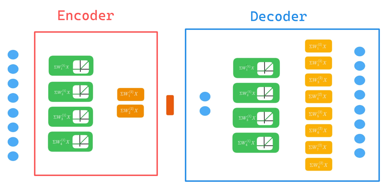
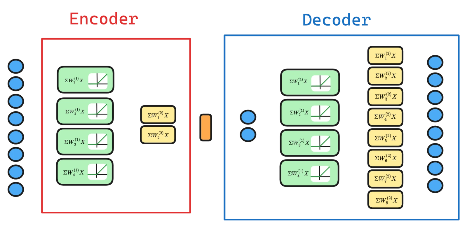 Figure 1.0: illustration of a classic Autoencoder neural network architecture.
After training, $z_1$ might separate high-value from low-value users and $z_2$ might separate active from churned — but those labels are never given. The geometry emerges from what the decoder needs to reconstruct.
No prior is placed on $z$. The latent space is organized however minimizes the loss — which makes autoencoders effective for anomaly detection (out-of-distribution inputs reconstruct poorly) but unreliable for generation (arbitrary points in $\mathcal{Z}$ decode to noise).
Reconstruction ≠ prediction — the encoder may retain high-variance but low-signal dimensions because they help reconstruction, while discarding low-variance but high-signal dimensions. A good reconstruction embedding is not necessarily a good predictive one.
3.2 Variational Autoencoders
An autoencoder finds a good compression, but nothing guarantees the latent space is organised. Two similar inputs may land in distant regions; a randomly sampled point decodes to noise because the decoder has never seen it.
A Variational Autoencoder (VAE) fixes this by encoding each input not as a single point but as a small cloud — a Gaussian distribution with learned mean and spread. The architecture remains encoder–decoder, but the encoder now outputs two vectors instead of one:
- Encoder outputs $\mu$ and $\sigma$ — for the user profile above: $\mu = [0.70,\; -1.20]$ (where this user most likely lives in $\mathcal{Z}$) and $\sigma = [0.15,\; 0.30]$ (how spread out the cloud is along each axis).
- Sampling — $z$ is drawn from $\mathcal{N}(\mu, \sigma^2)$, a different point each forward pass.
- Decoder — same role as before; reconstructs the input from the sampled $z$.
Intuition: because every input now occupies a region rather than a point, the clouds overlap. The gaps between training inputs are filled in. Random samples from $\mathcal{Z}$ decode to coherent outputs — generation becomes possible.
The reparameterization trick makes this trainable. Sampling from a distribution is not differentiable, so instead: draw noise $\varepsilon \sim \mathcal{N}(0, I)$ and construct $z$ deterministically:
\[z = \mu_\theta(x) + \sigma_\theta(x) \cdot \varepsilon\]Concretely (tabular): $\mu = [0.70,\; -1.20]$, $\sigma = [0.15,\; 0.30]$, draw $\varepsilon = [0.50,\; -0.80]$, giving $z = [0.775,\; -1.44]$. On the next pass a different $\varepsilon$ is drawn. From the optimizer’s perspective $\varepsilon$ is a constant, so gradients flow normally through $\mu$ and $\sigma$.
Visual example: on MNIST, each digit class occupies a fuzzy region rather than a point. Sampling between the “3” and “8” regions produces a smoothly morphed intermediate — a plain autoencoder cannot do this, as the interpolated region was never seen during training.
Why reconstruction loss alone is not enough. Minimizing $|x - \hat{x}|^2$ gives the encoder no reason to organise the space between training points. The result is a latent space that memorises positions but violates two properties needed for generation:
- Continuity — nearby points in $\mathcal{Z}$ should decode to similar outputs.
- Completeness — any point sampled from $\mathcal{Z}$ should decode to something meaningful.
Without a regularizer, the encoder is free to scatter clusters arbitrarily and leave dead zones between them. This is where the Kullback–Leibler divergence comes in.
KL Divergence as a Regularizer
KL divergence measures how one probability distribution $P$ diverges from a reference distribution $Q$:
\[D_{\text{KL}}(P \| Q) = \sum_i P(i) \log \frac{P(i)}{Q(i)}\]It is not a true distance — $D_{\text{KL}}(P | Q) \neq D_{\text{KL}}(Q | P)$ — but it captures the information cost of using $Q$ to approximate $P$. When $P = Q$, the divergence is zero; the more $P$ departs from $Q$, the larger it grows.
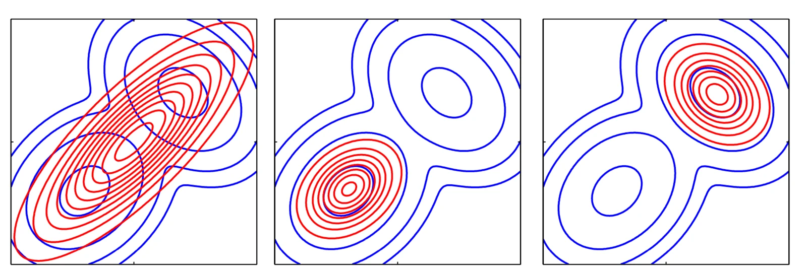 Figure 3.0: KL divergence fitting a simple distribution (red) to a complex one (blue). Left: identical distributions, $D{\text{KL}} = 0$. Centre and right: as the approximation concentrates on different modes, divergence increases. source_
In the VAE, $P$ is the encoder’s learned posterior $q_\theta(z \mid x)$ and $Q$ is the prior $\mathcal{N}(0, I)$. Minimizing $D_{\text{KL}}(q_\theta(z \mid x) | \mathcal{N}(0, I))$ forces every encoding cloud toward the origin with bounded spread — filling the gaps and ensuring continuity and completeness.
The training objective combines both terms as the Evidence Lower Bound (ELBO):
\[\mathcal{L} = \underbrace{\|x - \hat{x}\|^2}_{\text{reconstruction}} \;+\; \underbrace{D_{\text{KL}}\!\left(q_\theta(z \mid x) \;\|\; \mathcal{N}(0,I)\right)}_{\text{latent regularization}}\]The two terms are in tension. Reconstruction alone produces tight, scattered clusters with dead zones (left panel below). KL alone collapses everything into a single Gaussian — no structure survives (centre). The combination preserves class structure while keeping the space smooth and traversable (right).
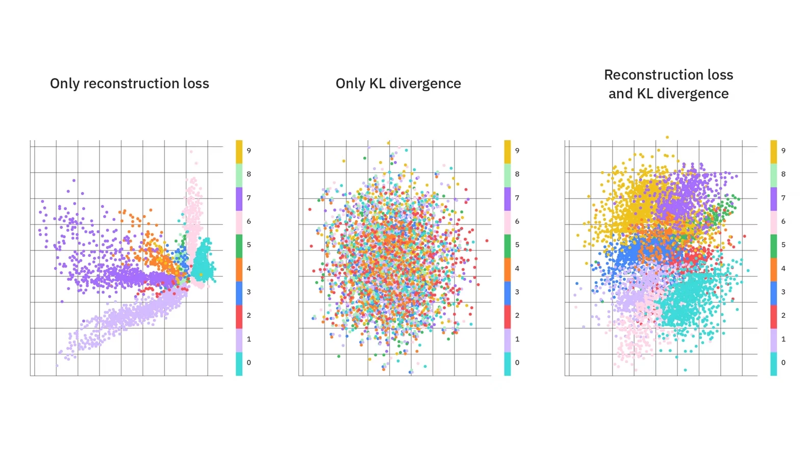 Figure 3.1: MNIST latent spaces trained with reconstruction loss only, KL divergence only, and both combined (ELBO). Only the combination produces a space that is both structured and complete. source
A scalar $\beta > 1$ on the KL term ($\beta$-VAE) pushes harder toward the prior — trading reconstruction fidelity for a more disentangled, tightly organised space; $\beta < 1$ relaxes toward the unregularised autoencoder.
| Property | Autoencoder | VAE |
|---|---|---|
| Latent $z$ | deterministic point | sampled from $(\mu, \sigma)$ |
| Latent structure | unregularized | regularized toward $\mathcal{N}(0,I)$ |
| Gradient through $z$ | direct | via reparameterization |
| Sampling new points | not meaningful | meaningful interpolation |
| Objective | reconstruction only | reconstruction + KL divergence |
3.3 A Note on Latent Space Geometry
All encoders above assume $\mathcal{Z} = \mathbb{R}^d$ — a flat Euclidean space. This is a structural assumption, not a necessity.
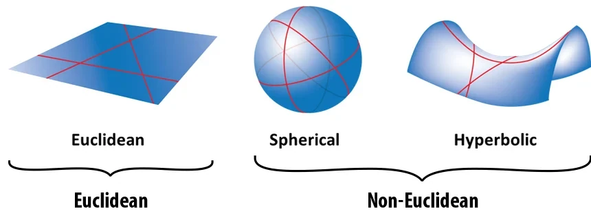 Figure 3.2: Euclidean, spherical, and hyperbolic geometries — each defines different geodesics and distance growth rates . source
In Euclidean space, geodesics are straight lines and distances grow linearly. In spherical space, geodesics curve back on themselves — suitable for data with cyclical structure. In hyperbolic space, space expands exponentially away from any center point — exactly matching the growth rate of trees and hierarchies.
This matters for embeddings: a tree with branching factor $b$ has $b^k$ nodes at depth $k$. Euclidean space cannot represent this exponential volume without distortion unless dimension grows proportionally. Hyperbolic space handles it natively in low dimension.
The Lorentz and Poincaré models are two equivalent ways to work with hyperbolic space computationally:
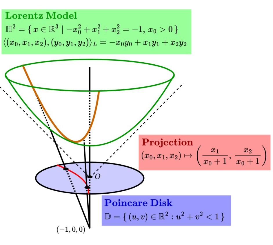 Figure 3.3: The Lorentz hyperboloid (left) projects onto the Poincaré disk (right) — boundary points are exponentially far from the center. source
The Lorentz model embeds hyperbolic space as a hyperboloid in $\mathbb{R}^{n+1}$:
\[\mathbb{H}^2 = \{ x \in \mathbb{R}^3 \mid -x_0^2 + x_1^2 + x_2^2 = -1,\; x_0 > 0 \}\]with inner product $\langle x, y \rangle_L = -x_0 y_0 + x_1 y_1 + x_2 y_2$. The Poincaré disk $\mathbb{D} = {(u,v) \in \mathbb{R}^2 : u^2 + v^2 < 1}$ is obtained by projecting the hyperboloid onto the unit disk. Points near the boundary of the disk are exponentially far from the center in hyperbolic distance — which is why hierarchical trees can be embedded with siblings close together and the root near the center, using very few dimensions.
Distance in the Poincaré ball model between two points $u, v$ is:
\[d_{\mathbb{B}}(u, v) = \text{arcosh}\!\left(1 + \frac{2\|u - v\|^2}{(1 - \|u\|^2)(1 - \|v\|^2)}\right)\]The denominator shrinks as points approach the boundary ($|u| \to 1$), so boundary-adjacent points are very far apart even if their Euclidean coordinates are close — the disk compresses exponential hyperbolic volume into a bounded region.
4. Positional Encoders
A Transformer has no built-in notion of order. Feed it “the cat sat on the mat” or “mat the on sat cat the” — it sees the same bag of tokens. Without help, every permutation is identical.
Positional encoders fix this by adding a position-dependent signal to each token before attention sees it. The token embedding carries what the word is; the positional encoding carries where it sits:
\[x'_t = x_t + PE(t)\]| Variant | How position enters | Learnable | Extrapolates to longer sequences |
|---|---|---|---|
| Sinusoidal (Vaswani 2017) | additive, fixed | no | yes (by design) |
| Learned absolute | additive lookup table | yes | no |
| RoPE | multiplicative rotation in attention | partially | yes |
| ALiBi | additive bias on attention scores | no | yes |
4.1 Sinusoidal Positional Encoding
The original Transformer uses a clever trick: encode each position $t$ as a $d$-dimensional vector built from sine and cosine waves at different frequencies — fast-changing waves for fine position, slow-changing waves for coarse position:
\[PE_{(t,\, 2i)} = \sin\!\left(\frac{t}{10000^{2i/d}}\right), \qquad PE_{(t,\, 2i+1)} = \cos\!\left(\frac{t}{10000^{2i/d}}\right)\]The table below makes this concrete. Dimensions 0–1 (high frequency) change dramatically between adjacent positions — they tell the model whether two tokens are one step apart. Dimensions 2–3 (low frequency) barely move at short range and only differentiate tokens across long spans.
Using both sine and cosine at each frequency is deliberate: it means any shift $PE(t + \Delta)$ can be written as a linear transformation of $PE(t)$, so the model can learn to compute “how far apart?” as a simple operation.
| Position | dim 0 ($\sin$, high freq) | dim 1 ($\cos$, high freq) | dim 2 ($\sin$, low freq) | dim 3 ($\cos$, low freq) |
|---|---|---|---|---|
| 0 | 0.000 | 1.000 | 0.000 | 1.000 |
| 1 | 0.841 | 0.540 | 0.010 | 1.000 |
| 2 | 0.909 | −0.416 | 0.020 | 1.000 |
| 3 | 0.141 | −0.990 | 0.030 | 1.000 |
| 4 | −0.757 | −0.654 | 0.040 | 0.999 |
The inner product $PE(t)^\top PE(t’)$ depends only on the offset $t - t’$, giving the model a built-in bias toward relative position. Since sinusoidal PE has no trainable components, it introduces zero estimation variance — its only bias comes from the design choice itself: the assumption that a fixed multi-frequency basis captures all the positional structure the model needs.
4.2 Relative and Rotary Variants
Modern large language models move position into attention rather than into token representations.
RoPE (Rotary Position Embedding) encodes position as a rotation applied to query and key vectors before computing attention. The rotation angle depends on the position difference, making attention scores inherently position-relative.
ALiBi (Attention with Linear Biases) adds a fixed negative slope to attention scores as a function of key-query distance — no vector modification required.
Both variants improve length generalization: a model trained on sequences of length 512 can be applied to sequences of length 2048 without degradation. This is where learned absolute PE fails — it introduces a trainable vector per position, so it has no representation for positions it never saw during training. RoPE and ALiBi sidestep this by encoding position as a relative offset rather than an absolute lookup, removing both the assumption bias of fixed sinusoids and the length generalisation variance of learned tables.
Positional encodings are not learned from labels — they are geometric injections. The model learns to use them; it does not learn what they are.
5. Semantic Encoders
Everything above encodes structure — categories, compressed data, position. Semantic encoders tackle a harder target: meaning. Given a sentence, a paragraph, or a document, they produce a representation that captures what the text is about, not just what symbols it contains.
The central question: how similar is A to B?
| Encoder type | Input | Output | Similarity computation |
|---|---|---|---|
| Bi-encoder | single text | dense vector | $f(q)^\top f(d)$ (dot product) |
| Cross-encoder | text pair $(q, d)$ | scalar score | full attention over the pair |
| Poly-encoder | query + multiple candidates | weighted sum | intermediate between the two |
5.1 Bi-Encoders
The simplest approach: encode the query and the document separately, then compare their vectors.
\[s(q, d) = f_\theta(q)^\top f_\theta(d)\]Because $f_\theta(d)$ can be precomputed for all documents, retrieval scales to billions of candidates via approximate nearest neighbor search.
Example: query “early symptoms of diabetes” → 768-dim vector $q$. Document “Fatigue and frequent urination are early signs of high blood sugar” → 768-dim vector $d$, computed once and stored. Similarity = $q^\top d = 0.87$. Nothing in this score knows that “early” in the query aligns with “early signs” in the document — the match is purely geometric, between two independently computed vectors.
The constraint is strong: each representation must be independently sufficient. The model cannot attend to tokens in $d$ while encoding $q$, so relationships that only emerge when query and document are read together are invisible to it — a structural bias built into the architecture. In exchange, document representations are computed once and reused for every query, eliminating the inference variance that comes from per-pair computation.
5.2 Cross-Encoders
What if the model could read both texts at once? A cross-encoder does exactly that — it concatenates query and document into a single input and processes them jointly:
\[s = f_\theta\bigl([q \,;\, \text{[SEP]} \,;\, d]\bigr)\]Every token in the query can now attend to every token in the document. “Symptoms” directly aligns with “signs”; “diabetes” with “blood sugar”. The model integrates these cross-attention alignments and outputs a single relevance score — much more precise than the dot product of two independent vectors, but only computable at query time.
| Property | Bi-Encoder | Cross-Encoder |
|---|---|---|
| Encoding | $f(q)$, $f(d)$ separately | $f([q; d])$ jointly |
| Precomputation | yes — index documents offline | no — must recompute per pair |
| Latency at query time | fast (ANN lookup) | slow (full forward pass per pair) |
| Expressivity | limited | high |
| Typical role | first-stage retrieval | second-stage reranking |
Cross-encoders remove the independence constraint, eliminating the structural bias that limits bi-encoders. The cost is that every query-document pair requires its own forward pass — no precomputation is possible, and the model is more sensitive to distributional shift between query and document populations.
In production retrieval systems, both are used in sequence: a bi-encoder retrieves a candidate set at scale, then a cross-encoder reranks the top candidates where precision matters.
Note that cross-encoders do not produce embeddings — they produce scores. The encoding is not a point in space; it is a function of a pair.
Conclusion
Most engineers think the model is where intelligence lives. It isn’t — it lives in the representation.
Once a categorical variable has been embedded into $\mathbb{R}^k$, the model can only reason within that geometry. It cannot undo an imposed order, rediscover collapsed identity, or remove leakage baked into expectation. The hypothesis space is shaped long before training begins.
If you cannot articulate the geometry your encoding imposes — the metric it defines, the assumptions it encodes — then you are not controlling your model. You are guessing at its world.
The model is not misunderstanding the data. It is faithfully executing the geometry you gave it.