Compute Infrastructure for ML Workloads

The software stack from kernel to container — drivers, compilers, runtimes, libraries, allocators, frameworks, serving, and orchestration

Posted May 20, 2026 Updated May 31, 2026

By ibrahim_lahlou

66 min read

Compute Infrastructure for ML Workloads

Overview

Machine learning systems feel deceptively simple from the outside.

You write a few lines of PyTorch, launch a training job, and somewhere beneath the API an enormous amount of machinery moves into place: kernels launch, memory pages move, DMA engines (dedicated hardware that moves data between devices without CPU involvement) push tensors across PCIe links, schedulers decide who gets compute time, distributed runtimes coordinate machines that may be continents apart.

Most of the time, you never see any of it.

The abstraction is designed that way. Modern ML tooling hides decades of systems engineering behind a remarkably small interface. But when performance collapses, VRAM runs out, GPUs idle unexpectedly, or scaling introduces strange bottlenecks, the abstraction starts to crack. The problem is no longer “inside PyTorch.” It lives somewhere deeper in the stack.

And that stack is older than machine learning itself.

The foundations come from operating systems, computer architecture, networking, and high-performance computing: Unix process models, virtual memory, PCIe, NUMA, compiler toolchains, distributed communication primitives. ML infrastructure did not replace these ideas — it inherited them, layered new abstractions on top, and repurposed them for a new kind of workload.

Understanding modern ML systems therefore means understanding where those layers meet, where they leak, and which one is actually responsible when something goes wrong.

This post walks through the stack from the bottom up: the layers underneath modern ML workloads, what each one owns, and how they interact in practice.

┌──────────────────────────────────────────────────┐
│ 9. Orchestration    Docker, Compose, K8s, Ray    │
│ 8. Serving          vLLM, TIS, TGI, Ray Serve    │
│ 7. Framework        PyTorch, JAX, MLX            │
│ 6. Allocator        caching allocator, cgroups   │
│ 5. Math libraries   cuBLAS, cuDNN, NCCL          │
│ 4. Runtime          libcudart, libcuda           │
│ 3. Compiler         nvcc, NVRTC, Triton DSL      │
│ 2. Driver           nvidia.ko, amdgpu.ko         │
│ 1. Kernel           syscalls, /proc, /sys        │
└──────────────────────────────────────────────────┘
              Hardware (CPU, RAM, GPU, NVMe)

1. The kernel layer

A Linux process never talks to hardware directly. It issues system calls into the kernel, and the kernel — through a driver — talks to the device. The reason is protection: every process has its own virtual address space (an isolated view of memory where addresses don’t directly map to physical RAM locations), and a misbehaving program cannot scribble on a PCIe device or another process’s memory because it has no way to even name them.

The kernel exposes its state through three surfaces:

/proc — per-process and kernel info as virtual files (/proc/cpuinfo, /proc/meminfo, /proc/PID/status).
/sys — device tree, driver parameters, cgroup controllers.
The ring buffer — a fixed-size circular buffer in kernel memory that stores chronological log of kernel events, read by dmesg. New messages overwrite old ones when full.

These are not real files. Reading them triggers a kernel callback that produces the answer on the fly, which is why cat /proc/cpuinfo is essentially free.

The ring buffer is where you go when something at the hardware layer is wrong:

  
dmesg -T --level=err,warn               # errors with timestamps
dmesg | grep -i -E 'nvidia|nvrm|amdgpu' # driver-related entries
dmesg | grep -i 'xid'                   # NVIDIA hardware faults

NVIDIA prints its own hardware error codes through the ring buffer, each tagged with a numeric ID called an Xid. Every Xid maps to a fault class — software bug, hardware fault, communication failure — and the mapping is stable across driver versions, so the same code in 2020 and in 2025 means the same thing. NVIDIA publishes the full table; the ones you will actually see are a handful: Xid 13 (grid sync timeout, an intra-GPU desync), Xid 31 (memory page fault — usually a software bug, occasionally failing memory), Xid 79 (the GPU fell off the PCIe bus — power or thermal). Anything in that family means stop tuning the model and go look at the hardware.

The same surface gives you CPU, RAM and disk visibility through dedicated tools that are just structured readers over /proc and /sys:

  
lscpu                            # sockets, cores, threads, NUMA, flags
free -h                          # mem total/used/available/cached
vmstat 1                         # paging activity per second
lsblk -o NAME,SIZE,ROTA,MODEL,TRAN  # block devices
iostat -xz 1                     # per-device IOPS, latency
numactl --hardware               # NUMA distances
lstopo --no-io                   # full topology, ASCII

Two lscpu outputs matter most for ML. The flags line tells you whether AVX-512, AVX10 or AMX (Intel matrix extensions) are available — PyTorch’s CPU kernels dispatch on these. And the NUMA (Non-Uniform Memory Access) section tells you how many memory nodes the box has. On dual-socket machines, each CPU socket has local RAM; every access from socket 0 to a DIMM on socket 1 crosses the inter-socket link (UPI [Ultra Path Interconnect, Intel’s socket-to-socket link] on Intel, Infinity Fabric on AMD) — 30 to 50 percent slower than local access due to additional hops and lower bandwidth. If data-loader threads sit on one socket and the GPU is on the PCIe root of the other, you pay this latency penalty on every batch:

  
numactl --cpunodebind=0 --membind=0 python train.py

Figure 1.0: A misplaced process reaching across UPI to remote memory

2. The driver layer

§1 stopped at the kernel boundary. The piece that translates between “kernel” and “this specific GPU” is the driver.

A driver is a kernel module — code that runs in kernel space (with full hardware access) and can be loaded or unloaded at runtime without rebooting, extending the kernel to speak to a specific class of device. On load it registers with the kernel’s device framework; the kernel then walks the PCIe bus (a tree structure connecting the CPU to all expansion devices), the driver binds to each device matching its vendor/device ID pair, and exposes them as files under /dev. Opening /dev/nvidia0 is how userspace attaches to the first GPU.

What people call “the NVIDIA driver” is four cooperating modules, each owning one concern:

nvidia.ko — core: command submission, on-GPU scheduler, VRAM management.
nvidia_uvm.ko — Unified Virtual Memory; CPU and GPU share an address space.
nvidia_drm.ko — Linux Direct Rendering Manager glue; the display-stack plug.
nvidia_modeset.ko — resolution, refresh rate, multi-monitor.

AMD bundles all of this into a single amdgpu.ko. Same end result, fewer modules.

Inspection commands walk the same path — modules, device nodes, version metadata:

  
lsmod | grep nvidia              # loaded modules
modinfo nvidia | head            # version, params, signature
ls /dev/nvidia*                  # nodes userspace opens
cat /proc/driver/nvidia/version  # driver self-report

The driver does not find the GPU — the kernel does, by walking PCIe at boot. PCIe is a tree (CPU root complex at the top, switches as branches, devices at the leaves); whichever driver claims a matching vendor/device ID gets bound to those nodes. lspci walks the same tree from userspace:

  
lspci -tv                        # tree view
lspci -vvv -s 01:00.0            # detail for one device
nvidia-smi topo -m               # GPU-GPU topology with NVLink (NVIDIA's high-bandwidth interconnect for direct GPU-to-GPU communication, bypassing PCIe and CPU)

PCIe is a negotiated interconnect. Every link has a width (number of lanes: x1, x4, x8, up to x16, where each lane is an independent serial connection) and a generation (Gen3 = 8 GT/s per lane, Gen4 = 16 GT/s, Gen5 = 32 GT/s, where GT/s = GigaTransfers per second; with 128b/130b encoding on Gen3+ this translates to roughly ~1 GB/s per GT/s per lane); the device, slot, and BIOS negotiate down to whatever they all support. In lspci -vvv, LnkCap is what the device can do, LnkSta is what got agreed. An x16 Gen5 GPU (128 GB/s bidirectional) in a slot the BIOS handed x8 Gen4 (32 GB/s) is an 8× bandwidth regression no software can fix.

One terminology trap, source of the most common ML-environment failure: “CUDA” is two things. A userspace toolkit (headers, compiler, runtime library) and a kernel-mode driver. They version independently, with one rule — newer driver supports older toolkit, never the reverse. This is forward compatibility: old binaries run on new drivers, but new binaries cannot run on old drivers (the toolkit may emit instructions the older driver doesn’t understand).

nvidia-smi reports the driver’s CUDA version (max toolkit it can run).
nvcc --version reports the toolkit’s CUDA version (what your code was compiled against).
They may disagree as long as driver ≥ toolkit.

nvidia-smi also exposes a few operational knobs. The one that matters for serving is persistence mode : by default the driver unloads when no CUDA process is running, and the next launch pays a 1–3 s reload. Invisible during a multi-hour training run, fatal for a low-traffic serving endpoint.

nvidia-smi -pm 1

nvidia-smi also sets the operating envelope — clocks, power cap, and on A100/H100/H200 whether the GPU is treated as one device or partitioned. MIG (Multi-Instance GPU) slices one A100/H100 into up to seven hardware-isolated instances, each with its own streaming multiprocessors (SMs — the GPU compute units), L2 cache partition, and dedicated HBM memory channels. This provides strict fault isolation for multi-tenant sharing — one instance’s error cannot crash another:

  
nvidia-smi -ac 1215,1410         # pin memory/SM clocks
nvidia-smi -pl 350               # power limit in watts
nvidia-smi mig -cgi 19,19,19 -C  # create 3 MIG slices

The same picture exists for AMD, with different names: rocm-smi, rocminfo, and /sys/class/kfd/ instead of the NVIDIA equivalents. For Apple Silicon there is no separate driver layer in this sense — the GPU shares unified memory with the CPU and is reached through Metal (Apple’s low-level graphics and compute API), which sits closer to a framework than a driver since CPU and GPU are on the same die.

A Windows remark: same concepts, different surfaces. Device Manager and pnputil replace lspci. The Event Viewer replaces dmesg. nvidia-smi works identically. WSL2 gives a full Linux userspace with GPU passthrough, which is what most people end up using. The rest of this post stays on Linux because that is where production ML lives.

2.1 GPU families and naming

A driver inspection prints something like “NVIDIA A100-SXM4-80GB” and assumes you can decode it. The string encodes lineage: architecture generation, market segment, board form factor, memory tier. The same software stack behaves very differently on a Turing T4 and a Hopper H100, and the model number is what flags it.

NVIDIA

NVIDIA names architectures after physicists and mathematicians. Each generation has a codename used in die designations (GA100, GH100) and a consumer-facing product line. The pattern: the architecture letter brands the datacenter card, the consumer brand stays GeForce, the trailing number sets the tier.

Architecture (year)	Die prefix	Datacenter flagship	Consumer / workstation
Fermi (2010)	`GF`	Tesla M2090	GeForce GTX 480 / 580
Kepler (2012)	`GK`	Tesla K80	GeForce GTX 680 / 780
Maxwell (2014)	`GM`	Tesla M40	GeForce GTX 980 / Titan X
Pascal (2016)	`GP`	Tesla P100	GeForce GTX 10xx / Titan Xp
Volta (2017)	`GV`	Tesla V100	Titan V
Turing (2018)	`TU`	Tesla T4	GeForce RTX 20xx / Quadro RTX
Ampere (2020)	`GA`	A100, A40, A30, A10	GeForce RTX 30xx, RTX A6000
Ada Lovelace (2022)	`AD`	L4, L40, L40S	GeForce RTX 40xx, RTX 6000 Ada
Hopper (2022)	`GH`	H100, H200, H800	(datacenter-only)
Blackwell (2024)	`GB`	B100, B200, GB200	GeForce RTX 50xx
Rubin (2026, planned)	`GR`	R100 (planned)	—

Product brands, decoded:

GeForce GTX — high-end consumer through Turing. The suffix started on GeForce 2 GTS, was reused on GeForce 8 GTX as a generic high-end marker, stuck for two decades.
GeForce RTX — same consumer line from Turing (RTX 20xx) on. “RT” = ray tracing; Turing was the first NVIDIA architecture with dedicated RT cores (ray-triangle intersection) and Tensor Cores (matmul) alongside shaders.
Quadro / RTX A-prefix — workstation cards. Same silicon as GeForce, but with ECC, ISV-certified drivers, FP64 enabled. “Quadro” was retired in 2020; current workstation cards are “RTX A6000” (Ampere) and “RTX 6000 Ada”.
Tesla — original datacenter brand (2007–2020). K80, P100, V100. Retired from Ampere on; the architecture letter does the branding now and the car company stopped sharing the name.
A / H / B-series datacenter — A100 = Ampere, H100 = Hopper, B100 = Blackwell. The architecture letter is the brand. Trailing number is the tier: 100 flagship (large die, NVLink, SXM); 200 enhanced refresh (H200 = H100 with HBM3e); 40 midrange PCIe; 30 / 10 lower-tier inference.
L-series — Ada Lovelace datacenter, inference-aimed: L4 (72 W, single slot), L40 / L40S (full-height). Same Ada die as RTX 6000 Ada, FP64 disabled to cut cost. “L” = Lovelace, parallel to how “T” = Turing.
T-series — Turing datacenter, in practice just the T4. 70 W INT8/INT4 inference workhorse, still everywhere five years on.
Titan — discontinued enthusiast line above GeForce (Titan X, Titan V, Titan RTX). The pre-2020 ML escape hatch when datacenter cards were unobtainable; replaced by the RTX xx90 tier.
Jetson — embedded edge (Nano → Orin → Thor). Same CUDA stack, ARM CPU and GPU on one SoM.
-800 suffix — China-export variants (A800, H800, H20). Same die, NVLink bandwidth capped to stay under US export thresholds.

Reading the names back: “A100-SXM4-80GB” = Ampere, top tier (100), SXM4 board (Server PCI eXpress Module: a proprietary socket form factor for datacenter GPUs, not a PCIe slot; enables NVLink and higher power delivery than PCIe), 80 GB HBM2e. “RTX 4090” = RTX consumer, Ada Lovelace (40-series), top SKU (90). “L40S” = Lovelace datacenter, midrange (40), “S” refresh.

AMD

AMD split its GPU architecture into two lineages in 2020: consumer graphics (RDNA) and datacenter compute (CDNA). Shared ROCm stack, no shared microarchitecture.

Architecture	Year	Consumer (Radeon RX)	Datacenter (Instinct MI)
GCN 1–5	2012–2019	RX 200 / 300 / 400 / 500	MI8, MI25, MI50, MI60
RDNA / RDNA 2	2019–2020	RX 5000 / 6000	—
CDNA	2020	—	MI100
RDNA 3	2022	RX 7000	—
CDNA 2 / CDNA 3	2021–2023	—	MI200 series, MI300X
RDNA 4	2025	RX 9000	—
CDNA 4	2025	—	MI325X, MI355X

Names, decoded:

Radeon — AMD’s GPU umbrella since 2000 (post-ATI acquisition).
Radeon RX — consumer gaming line from 2016. “RX” started as “Radeon eXperience”; now just a brand mark.
Radeon Pro — workstation (Pro W7900). Certified drivers, ECC, more memory than equivalent RX.
Instinct MI — datacenter / HPC. “MI” is part of the model number, not formally expanded by AMD but widely read as “Machine Intelligence”. MI300X (CDNA 3, 192 GB HBM3) is the current deployed flagship; MI325X and MI355X are CDNA 4 successors.
CDNA vs RDNA — Compute DNA vs Radeon DNA. CDNA drops graphics-only blocks (rasterizer, display engine) to spend the area on more compute units and HBM controllers; RDNA keeps them and tunes for gaming.

Apple Silicon

Apple Silicon does not separate CPU and GPU at the package level — the GPU sits on the same die, sharing unified memory with the CPU, Neural Engine, and media blocks. No Linux-style driver; the GPU is reached through Metal or via MLX (the ML framework wrapping it).

Each M-series generation comes in tiers — base, Pro, Max, and on some generations Ultra. The tier sets GPU core count, memory-bus width, and max unified memory.

Generation (year)	Base GPU cores	Pro GPU cores	Max GPU cores	Ultra GPU cores	Max unified memory
M1 (2020)	7–8	14–16	24–32	48–64	128 GB
M2 (2022)	8–10	16–19	30–38	60–76	192 GB
M3 (2023)	8–10	14–18	30–40	(no Ultra)	128 GB
M4 (2024)	8–10	16–20	32–40	(no Ultra yet)	128 GB
M5 (2025)	10	TBA	TBA	—	TBA

Tier naming:

base M — entry chip; MacBook Air, iPad Pro, base Mac mini.
M Pro — wider memory bus (≈200–270 GB/s), more GPU cores; 14”/16” MacBook Pro.
M Max — much wider bus (≈400–550 GB/s), double the Pro’s GPU cores; large MacBook Pro and Mac Studio.
M Ultra — two Max dies fused via “UltraFusion”. Doubles bandwidth (~800 GB/s) and cores again; Mac Studio / Mac Pro only.

The Max and Ultra tiers are where Apple matters for ML. An M4 Max with 128 GB unified memory holds a 70 B model in 4-bit at usable rates with no offloading — the GPU has direct access to all 128 GB at ~500 GB/s. No discrete consumer NVIDIA card matches that capacity at any price.

3. The compiler layer

§2 made the GPU addressable. Now the question is how source code becomes something the GPU can execute — GPUs run their own ISA, and there has to be a compiler chain that crosses the gap.

Three NVIDIA compilers participate, each existing for a different reason:

nvcc — ahead of time. Invoked from a Makefile when you build a CUDA C++ project. Runs once at build time.
NVRTC — runtime, in-process, takes a CUDA C++ string. Exists so frameworks like PyTorch can generate kernels on the fly and cache them.
Triton DSL — kernel language embedded in Python with its own compiler. Exists so library authors can write GPU kernels without dropping into CUDA C++.

A modern PyTorch program uses all three at once — nvcc-built host code, NVRTC-compiled kernels from torch.compile, Triton-compiled kernels from Flash Attention.

3.1 nvcc and the host compiler

A .cu file is mixed: host code (CPU C++ that sets up data and launches kernels) and device code (__global__ / __device__ functions that run on the GPU). This split exists because the CPU and GPU have different instruction sets and memory spaces. Neither compiler understands the other half. nvcc is the dispatcher that splits the input and routes each half:

foo.cu ──┬─→ host C++   ──→ gcc / clang / msvc ──→ host .o ──┐
         │                                                    ├──→ executable
         └─→ device C++ ──→ cicc ──→ PTX ──→ ptxas ──→ SASS  ┘

Two intermediate forms appear in the pipeline, named because they show up constantly in errors and diagnostics:

PTX (Parallel Thread eXecution) — NVIDIA’s virtual ISA (instruction set architecture). Architecture-independent, like LLVM IR or JVM bytecode. Not what the GPU runs directly.
SASS (Streaming Assembler) — real GPU machine code, specific to a single compute capability (the GPU’s architecture version). What the SM (streaming multiprocessor, the GPU’s compute unit) executes.
fatbin — a “fat binary” container wrapping multiple SASS targets plus a PTX fallback in one artifact, allowing one binary to run on multiple GPU architectures.

PTX exists for forward portability: SASS for Ampere cannot run on Hopper, but PTX can be JIT-compiled (just-in-time: compiled at runtime, not build time) to SASS for whatever GPU is present. Every NVIDIA GPU advertises a compute capability (sm_XX) naming which SASS instructions it understands:

GPU	Capability	`nvcc` flag
V100	7.0	`sm_70`
T4 / RTX 20xx	7.5	`sm_75`
A100	8.0	`sm_80`
RTX 30xx	8.6	`sm_86`
RTX 4090 / L40	8.9	`sm_89`
H100 / H200	9.0	`sm_90`
B100 / B200	10.0	`sm_100`
RTX 50xx	12.0	`sm_120`

A production build embeds SASS for every target you care about plus a PTX fallback:

  
nvcc -O3 \
  -gencode arch=compute_80,code=sm_80 \
  -gencode arch=compute_89,code=sm_89 \
  -gencode arch=compute_90,code=sm_90 \
  -gencode arch=compute_90,code=compute_90 \  # PTX fallback
  kernel.cu -o app

The trailing compute_90,code=compute_90 embeds PTX. If the GPU at runtime is newer than every embedded SASS, the driver JIT-compiles the PTX to native (a one-time 1–5 s pause, cached afterward). This is how a PyTorch wheel built against CUDA 11.8 still runs on Blackwell.

Host compiler coupling. nvcc hands host code to gcc / clang / MSVC, and that compiler’s version must be on CUDA’s supported list. Mismatches produce errors that look like C++ standard-library bugs but are actually toolchain mismatches:

CUDA	gcc supported	clang supported
11.8	6.x – 11.x	up to 14
12.4	6.x – 13.x	up to 17
13.2	8.x – 14.x	up to 19

  
nvcc -ccbin /usr/bin/g++-12 kernel.cu   # pin host compiler explicitly
nvcc -Xcompiler "-fopenmp,-fPIC,-march=native" \
     -Xptxas "-v,-O3" \                 # -v prints reg/shmem usage
     -std=c++17 kernel.cu -o app

-Xptxas -v is the most useful flag during kernel tuning — it prints per-kernel register count and shared-memory footprint, which directly determines occupancy. Occupancy is the ratio of active warps to maximum possible warps on an SM. A warp is a group of 32 threads that execute the same instruction simultaneously (SIMT: Single Instruction, Multiple Threads). Higher occupancy means more warps to hide memory latency — when one warp stalls waiting for memory, another can execute.

The nvcc family:

ptxas — assembles PTX to SASS, tuned via -Xptxas.
cuobjdump, nvdisasm — inspect fatbins, dump SASS.
nvprune — strip unused architectures to shrink wheel size.
hipcc — ROCm’s analog, wrapping clang with the AMDGPU backend.

Figure 2.0: The host/device split and PTX-to-SASS pipeline

3.2 NVRTC — runtime compilation

nvcc works when kernels are fixed at build time. Modern frameworks aren’t: torch.compile synthesizes a kernel per model shape, and shipping a plugin wheel cannot know the target GPU in advance. Build-time is too late; you need a compile step at runtime.

NVRTC (libnvrtc.so) takes a CUDA C++ source string in memory, compiles it to PTX in-process, hands it back so the driver can JIT to SASS. No nvcc subprocess, no temp files. Used by TorchInductor, CuPy inline kernels, and plugin systems injecting custom ops.

Cost is one JIT compile per kernel per process — ms to seconds. Both PyTorch and CUDA cache the result (~/.cache/torch/inductor, ~/.nv/ComputeCache); the first run after a driver or PyTorch upgrade recompiles everything, which is why it feels slow with no model change.

3.3 Triton DSL — kernels in Python

NVRTC solves the when (compile at runtime). Triton DSL solves the what: CUDA C++ is verbose and forces you to manage warps, shared memory, and tensor cores by hand. Triton (originally OpenAI’s, distinct from NVIDIA’s Triton Inference Server in §8) is a Python-embedded DSL where you describe kernels in blocks (tiles of work) and let the compiler handle warp scheduling, shared-memory allocation, and tensor-core dispatch.

A minimal element-wise add:

  
import triton
import triton.language as tl

@triton.jit
def add_kernel(x_ptr, y_ptr, out_ptr, n_elements, BLOCK_SIZE: tl.constexpr):
    pid = tl.program_id(axis=0)
    offsets = pid * BLOCK_SIZE + tl.arange(0, BLOCK_SIZE)
    mask = offsets < n_elements
    x = tl.load(x_ptr + offsets, mask=mask)
    y = tl.load(y_ptr + offsets, mask=mask)
    tl.store(out_ptr + offsets, x + y, mask=mask)

The compiler underneath has shifted (originally clang-based, MLIR-based since 2023 — MLIR is a compiler infrastructure for building reusable compiler components), but the lowering ends the same place: Triton IR → PTX → SASS, same back end as nvcc.

This is where most of the modern ML kernel layer is written: Flash Attention’s reference impl, Mamba, the bulk of vLLM’s custom kernels, most of torch.compile’s generated code. The right abstraction when CUDA C++ is too low-level and PyTorch ops are too coarse — which is where most novel kernels live.

4. The runtime layer

§3 produced GPU machine code. The runtime layer loads it, hands it to the driver, schedules it onto a GPU, tracks memory — a thin userspace library between the compiled code and the kernel-mode driver.

CUDA exposes this as two stacked libraries (not alternatives):

libcuda.so — driver API . Low-level, stable across CUDA versions, shipped with the driver. Every CUDA process opens it first.
libcudart.so — runtime API . Higher-level wrappers, version-tied to the toolkit. What your CUDA C++ code links against by default.

The driver API has to be stable; the higher-level layer evolves alongside the toolkit.

Before launching anything, a process sets up a CUDA context: per-device, per-process state that includes GPU-side page tables (mapping virtual to physical VRAM addresses), command queues (lists of kernels waiting to execute), and a default stream (the execution queue kernels go to unless you specify otherwise). PyTorch dlopens libcuda.so, allocates a context per device, then it can launch kernels. Context creation costs 1–3 s on a cold GPU; persistence mode (§2) keeps the driver loaded to avoids paying this cost per process.

Once a context exists, four runtime concepts show up in ML code:

Streams — independent command queues on the GPU. GPU work is asynchronous: the CPU launches kernels into a stream and continues without waiting. Kernels in different streams may run concurrently (if resources allow); kernels in the same stream execute sequentially. The default stream is stream 0, created automatically; torch.cuda.Stream() creates additional ones for overlapping compute with data transfers.
Events — sync markers placed inside a stream, used to wait or measure. torch.cuda.Event(enable_timing=True) records GPU timestamps for profiling.
Graphs — captured kernel-launch sequences replayed as one submission. Removes per-launch CPU overhead (~5 μs per kernel × hundreds of kernels = significant waste). Critical for decode loops where the same kernels run repeatedly.
Memory — cudaMalloc, cudaMallocAsync, cudaMallocManaged (unified virtual addressing where CPU/GPU share one address space), cudaHostAlloc (page-locked). The framework’s caching allocator (§6) sits on top.

  
import torch

# CUDA Graph capture for a decode step
g = torch.cuda.CUDAGraph()
with torch.cuda.graph(g):
    out = model(static_input)
g.replay()  # near-zero CPU overhead

CUDA Graphs matter more than the name suggests. Each LLM decode token launches ~50–200 kernels (per-layer norms, projections, attention, MLP), each launch costs ~5 μs of CPU overhead (validation, arg copy, queue push). At 50 tok/s that’s up to 50 ms/s of wall time — ~5% — spent on launch overhead unrelated to the math. Capturing the step collapses those launches into one submission, removing the overhead. vLLM, TensorRT-LLM, and SGLang all rely on it.

5. The math library layer

§4 gave you the ability to launch a kernel, not a kernel worth launching. A useful matmul, FFT, or convolution is dozens of pages of architecture-specific code — tile sizes, Tensor Cores, shared-memory swizzling (reordering memory layout to avoid bank conflicts: when multiple threads in a warp try to access the same shared memory bank simultaneously, causing serialization), HBM latency hiding. Almost nobody writes these by hand. The math libraries are the vendor-tuned versions, refreshed per generation, and they are the practical performance ceiling — every framework links against them rather than rolling its own.

NVIDIA’s library surface, by primitive:

Library	Operations	Used by
cuBLAS / cuBLASLt	GEMM (GEneral Matrix Multiply), batched GEMM, mixed precision. cuBLASLt = “Lightweight” with finer control over epilogue fusion (fusing ops like bias add, activation, scaling into the matmul kernel so the intermediate result never leaves GPU registers)	every framework’s linear/matmul
cuDNN	Convolutions, RNN, attention primitives	CNNs, some transformers
CUTLASS	CUDA Templates for Linear Algebra Subroutines: C++ template library providing modular GEMM components (tiling, warp specialization, epilogue) you compose to build custom high-performance kernels	Flash Attention, custom ops
cuFFT	FFTs (Fast Fourier Transforms)	signal/audio, diffusion timestep ops
NCCL	All-reduce, all-gather, broadcast across GPUs	DDP, FSDP, TP, EP
cuSPARSE	Sparse matmul	sparse models, some MoE routing
TensorRT	Full inference graph optimizer, fused kernels	production inference

Three properties drive real optimization decisions, with silent failure modes — code still runs, just slowly:

Tensor Cores have alignment rules. Tensor Cores are specialized matrix-multiply units inside each SM (streaming multiprocessor), separate from the general-purpose CUDA cores, designed for deep learning workloads. Each generation supports different dtypes:
- TF32 (TensorFloat-32): 19-bit format (8-bit exponent like FP32, 10-bit mantissa) that fits in 32 bits with 10 bits of padding. Same range as FP32, less precision. Ampere+ default for FP32 inputs to Tensor Cores.
- BF16 (Brain Float 16): 16-bit format matching FP32’s 8-bit exponent, 7-bit mantissa. Same range, much less precision. Good for training.
- FP16: IEEE half-precision, 5-bit exponent, 10-bit mantissa. Narrower range than BF16 but more precision.
- FP8 E4M3/E5M2: 8-bit formats for H100+. E4M3 = 4-bit exponent, 3-bit mantissa (more precision). E5M2 = 5-bit exponent, 2-bit mantissa (more range, for gradients).
cuBLAS only dispatches to Tensor Cores when matrix dimensions are multiples of 8 (FP16) or 16 (INT8). Off-by-a-few shapes silently fall back to CUDA cores — 5× perf cliff for what looks like a typo.
cuDNN picks algorithms per shape. Many variants per convolution, chosen via heuristics or benchmark on first call. Cached, but every new shape re-triggers selection — why dynamic shapes hurt.
NCCL picks its transport from topology. Reads nvidia-smi topo -m at init and chooses a reduction tree matching the physical layout. NCCL_DEBUG=INFO to print the choice, NCCL_P2P_DISABLE=0 to force NVLink P2P, NCCL_IB_HCA to bind a specific InfiniBand card (InfiniBand: high-speed, low-latency networking for HPC and multi-node training).

  
NCCL_DEBUG=INFO NCCL_DEBUG_SUBSYS=ALL torchrun --nproc-per-node=8 train.py

The classic silent failure at this layer: NCCL ends up using TCP/IP between two NVLink-connected GPUs because of a kernel module misconfig, missing IPC (Inter-Process Communication: GPU peer-to-peer access where one process’s GPU can directly read another process’s GPU memory) permission, or a misdirected NCCL_* env var. Training “works” — gradients flow, loss decreases — but throughput drops 10×. Fix: turn on NCCL_DEBUG=INFO, read the chosen transport, chase the discrepancy.

6. The allocator layer

§4 gave us cudaMalloc. No production framework calls it directly — two reasons. It’s slow (synchronous with the device: the CPU must wait for the GPU to acknowledge the allocation before continuing, hundreds of microseconds per call, forever in a loop allocating thousands of tensors per step), and naive use fragments VRAM badly because the driver’s device-side allocator wasn’t designed for high-churn workloads.

Every framework converges on the same fix: a userspace caching allocator between the framework and cudaMalloc. PyTorch’s is the canonical one, and it shows up in every OOM message you’ll see.

6.1 The PyTorch caching allocator

The allocator runs a memory pool: asks the driver for large VRAM slabs, carves them into blocks on demand, reuses freed blocks instead of returning them. The sequence on tensor.cuda():

Round the request up to a bucket size (powers of two, roughly).
Look for a free block in that bucket.
If found, return it. If not, ask cudaMalloc for a larger segment and split it.
On del tensor, the block returns to the pool — it is not returned to the driver.

This is why nvidia-smi reports more memory used than torch.cuda.memory_allocated(). Three numbers describe the state:

  
torch.cuda.memory_allocated()      # actively used by live tensors
torch.cuda.memory_reserved()       # held by PyTorch's pool
torch.cuda.max_memory_allocated()  # high-water mark
print(torch.cuda.memory_summary()) # full breakdown by bucket

6.2 Fragmentation — when allocation fails despite free memory

The classic OOM that confuses new users: nvidia-smi shows 20 GB free, PyTorch reports memory_allocated() of 30 GB on an 80 GB GPU, and a 5 GB allocation fails with CUDA out of memory. Tried to allocate 5.00 GiB. The free memory exists but is fragmented across many small blocks — no single contiguous 5 GB region.

This happens whenever allocation sizes vary across iterations: variable sequence lengths, dynamic batches, attention with KV cache. Two mitigations:

  
export PYTORCH_CUDA_ALLOC_CONF=expandable_segments:True

expandable_segments (added in PyTorch 2.1) lets the allocator grow segments instead of allocating fixed-size ones, dramatically reducing fragmentation for variable workloads. It is what vLLM uses by default.

  
export PYTORCH_CUDA_ALLOC_CONF=max_split_size_mb:128

max_split_size_mb caps how large a block can be split into smaller pieces, preventing big segments from being chopped up irreversibly.

If you suspect fragmentation, dump the snapshot:

  
torch.cuda.memory._record_memory_history()
# ... run workload ...
torch.cuda.memory._dump_snapshot("snap.pickle")
# load in https://pytorch.org/memory_viz to visualize

6.3 Page-locked (pinned) memory

GPU allocation is half the story. The other half is getting data to the GPU, every batch — disk → host RAM → VRAM. The host RAM step has a slow default.

By default, the host buffer is pageable: the OS can move those virtual memory pages to different physical RAM locations or swap them to disk, and the GPU’s DMA engine (hardware that copies data between devices) can’t read from non-fixed physical addresses — it needs stable physical locations. The driver works around this with a staging buffer: pageable host memory → driver-owned page-locked buffer → device. That intermediate copy is wasted bandwidth.

The fix is to allocate the host buffer as pinned via cudaHostAlloc, which locks the pages. The DMA engine then copies directly host→VRAM, skipping the staging hop. In PyTorch:

  
loader = DataLoader(dataset, pin_memory=True, num_workers=8)
# inside the loop:
batch = batch.to(device, non_blocking=True)  # async copy from pinned host

Trade-off: pinned pages can’t be paged out, so they count against physical RAM permanently. Over-pinning starves the system. Pin the data loader’s output, not much else.

6.4 cgroups — the kernel’s resource governor

Everything in §6 so far is userspace. Below it, the kernel enforces per-process memory and CPU limits via cgroups v2 (control groups: a Linux kernel feature for organizing processes into hierarchical groups with resource limits). Every container, systemd service, and nice-d shell sits in one whether you set it up or not. The cgroup is what eventually OOM-kills a process that thinks it has more RAM than it really does.

Controllers relevant to ML:

Controller	Limits
`memory`	RAM, swap, OOM behavior
`cpu`	CPU shares, quota
`cpuset`	Which cores and NUMA nodes a process may use
`io`	Block-device bandwidth and IOPS
`pids`	Max processes (matters for DataLoader workers)

  
# inspect a container's cgroup
cat /sys/fs/cgroup/memory.max
cat /sys/fs/cgroup/cpuset.cpus.effective

# pin a training run to socket 0 cores and memory node 0
systemd-run --scope -p AllowedCPUs=0-31 -p AllowedMemoryNodes=0 \
  python train.py

GPU memory is not cgroup-controlled in mainline kernels. The driver enforces per-process limits internally; containers see GPUs through device passthrough, not cgroup quotas. This is why a process can OOM the GPU without tripping any container memory limit.

Figure 3.0: The five layers between tensor.cuda() and physical VRAM

7. The framework layer

§1–§6 are pieces the framework sits on top of: kernel, driver, compiler chain, runtime, vendor math libraries, allocator. The framework stitches them into something a researcher writes code against — owning the tensor API, autograd (automatic differentiation: computing gradients by recording a computational graph and applying the chain rule backward through it), op-dispatch logic, model parallelism, and increasingly its own compiler.

Three frameworks matter for compute-heavy ML today: PyTorch, JAX, MLX. Same design space, different choices about when execution happens, how the graph is captured, how autograd is wired, and how compilation interacts.

Framework	Execution	Compilation	Distributed
PyTorch	Eager by default	`torch.compile` (TorchInductor → Triton DSL)	DDP (DistributedDataParallel: replicate model, shard data, all-reduce gradients), FSDP (Fully Sharded Data Parallel: shard model + optimizer state + gradients), TP via DTensor (Distributed Tensor: abstraction for sharded tensors with automatic resharding)
JAX	Lazy / traced	XLA (HLO → LLVM/PTX)	pjit, sharding annotations
MLX	Lazy, unified memory	Built-in, no separate compile step	None for multi-machine

PyTorch is eager by default — every operation executes immediately when called, returning concrete values you can inspect in Python; pdb works naturally. The cost is no cross-op fusion (combining multiple operations into one kernel). torch.compile is the answer: trace once (record what operations run), lower through TorchInductor to Triton DSL kernels, replay the optimized graph on every subsequent call.

  
import torch
model = torch.compile(model, mode="reduce-overhead")  # captures CUDA Graphs
out = model(x)  # first call slow, rest fast

The mode argument is the main knob. mode="reduce-overhead" captures into a CUDA Graph (§4) — useful for short repeated runs like LLM decode where launch overhead dominates. mode="max-autotune" turns on aggressive Inductor autotuning including Triton kernel config search: very slow first run, faster steady state, worth it for long jobs.

JAX is lazy by default — every operation is recorded as a node in a computational graph rather than executing immediately; nothing actually runs until you call jax.jit (just-in-time compile and execute). The trace goes to XLA, lowered through HLO (High-Level Optimizer IR) → LLVM IR → PTX. Stricter than PyTorch: shapes must be static at compile time, control flow must use special ops (jax.lax.cond / scan / while_loop) instead of Python if/for. The payoff is some of the best fused kernels for matmul-heavy workloads, which is why Google’s TPU code lives in JAX.

MLX is Apple’s, and it skips the explicit compile step. Lazy graph like JAX, but executed by mx.eval with no JIT decorator exposed. The interesting property is unified memory: no host-device copy because the GPU shares physical memory with the CPU. An M3 Ultra with 128 GB runs a 4-bit-quantized 70 B model at usable rates with no offloading — a scenario no discrete GPU matches at any price.

7.1 Counting work: FLOPs and arithmetic intensity

A FLOP is one floating-point operation. By convention a fused multiply-add (FMA: computes $a \cdot b + c$ in one instruction) — one multiply and one add executed atomically — counts as 2 FLOPs, because that is the work that would otherwise be done by two scalar ops. Modern GPUs and CPUs have FMA units; Tensor Cores are specialized FMA units that operate on entire matrix tiles simultaneously. Tensor Cores execute a matrix-multiply-accumulate $D = A \cdot B + C$ on a tile (8×4×8 on Ampere using WMMA [Warp Matrix Multiply-Accumulate: PTX instructions where a warp cooperates to compute one tile], larger tiles on Hopper using WGMMA [Warpgroup MMA: 4 warps cooperate on larger tiles]) per warp per cycle; the FLOP count is the product of the tile’s $M \cdot N \cdot K$ times 2 (times 2 because each multiply-add is 2 FLOPs).

For a dense transformer with $N$ parameters processing $T$ tokens (Kaplan et al. 2020, Scaling Laws):

\[\text{FLOPs}_{\text{forward}} \approx 2NT, \quad \text{FLOPs}_{\text{train step}} \approx 6NT\]

The 2 = one multiply + one add per parameter per token. The 6 = forward + backward (~2×) + optimizer (~1×). This ignores the attention term, which dominates at long context:

\[\text{FLOPs}_{\text{attn}} \approx 4 L H_{kv} d_h S^2 B\]

with $L$ layers, $H_{kv}$ KV heads, $d_h$ head dim, $S$ sequence length, $B$ batch.

The theoretical ceiling. Every GPU has a fixed peak FLOPS — SM count × clock × FLOPs-per-cycle for that dtype. It is the wall no kernel can break:

\[\text{FLOPS}_{\text{peak}} = N_{\text{SM}} \cdot f_{\text{clock}} \cdot \text{ops}_{\text{cycle/SM}}\]

GPU	FP32	TF32 (TC)	BF16/FP16 (TC)	FP8 (TC)	FP4 (TC)	HBM BW
A100 80 GB	19.5	156	312	—	—	2.0 TB/s
H100 SXM	67	495	989	1979	—	3.35 TB/s
H200 SXM	67	495	989	1979	—	4.8 TB/s
B100	~80	~900	1800	3500	7000	8 TB/s
B200	~90	~1125	2250	4500	9000	8 TB/s

(TFLOPS, dense Tensor Cores; structured-sparsity throughput is ~2×. Structured sparsity = 2:4 pattern where 2 out of every 4 consecutive weights are zero, enabling Ampere+ Tensor Cores to skip zero-multiplies and double throughput. HBM = High Bandwidth Memory, the GPU’s on-package VRAM.)

These numbers are aspirational. The H100’s 989 BF16 TF/s assumes every SM runs a Tensor Core MMA every cycle with zero memory stalls, zero instruction overhead, and perfect tile alignment. Production training lands at 40–55%; that ratio is MFU.

The closed-form lower bound on a step time is straightforward:

\[T_{\text{step}}^{\text{min}} = \frac{6 N T}{\text{FLOPS}_{\text{peak}} \cdot \text{MFU}}\]

If a 70B model training on 8×H100 with MFU 0.45 takes 4× longer than this formula predicts, the rest is communication, data loading, or stalls — not compute. Walk the stack.

Tool	Type	Notes
`calflops`	Static trace	pip-installable
`fvcore.nn.FlopCountAnalysis`	Static trace	Meta, Detectron2
`ptflops`	Static trace	older
DeepSpeed `flops_profiler`	Static + dynamic	training loop
Nsight Compute	Hardware counters	`sm__sass_thread_inst_executed_*`
PyTorch profiler	Hardware counters	`with_flops=True`

Public benchmark sites for comparing models/hardware: artificialanalysis.ai, llm-stats.com, mlcommons.org/benchmarks/inference, the LMSYS leaderboard.

MFU (Model FLOPs Utilization) = achieved FLOPS / peak FLOPS. Production training: 40–55% on H100 is excellent. Below 30% means memory-bound (waiting for data from HBM, not enough compute to hide latency) or communication-bound (waiting for network/NVLink transfers), not compute-bound (waiting for arithmetic units) — fix that before tuning kernels.

The companion metric is arithmetic intensity — FLOPs per byte loaded from HBM. The roofline model says the achievable throughput is $\min(\text{peak FLOPS}, \text{intensity} \times \text{HBM bandwidth})$. Below a critical intensity (~290 on H100 for BF16), you are memory-bound (bottlenecked by how fast you can load data); above, compute-bound (bottlenecked by how fast you can perform arithmetic operations). Decode is far below (loads many weights per token); prefill is far above (reuses weights across many tokens). Knowing which side you are on determines what to optimize.

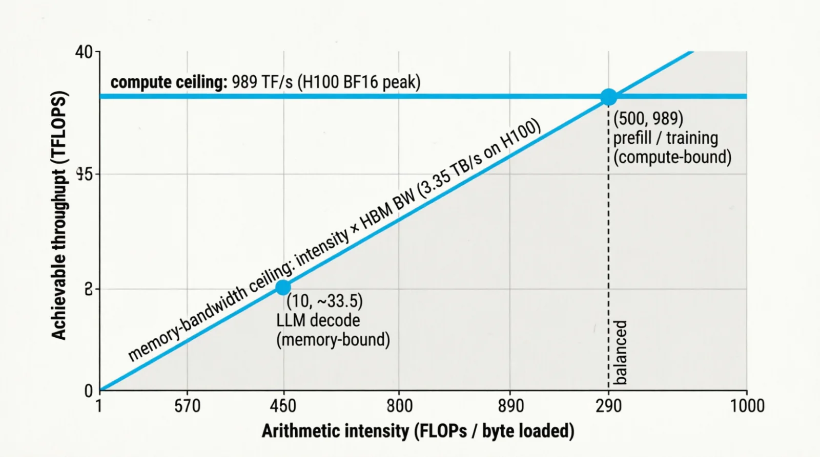Figure 4.0: The roofline — peak FLOPS as the ceiling, HBM bandwidth as the slope

8. The serving layer

For training, the framework is enough — torchrun, FSDP, that is the toolchain. For serving, there is a separate layer of software whose only job is to wring throughput from a fixed model. Three pieces dominate: vLLM (the engine), NVIDIA Triton Inference Server (the multi-framework runtime — different thing from Triton DSL), and Ray Serve (the routing layer that orchestrates everything).

8.1 The inference metric taxonomy

Inference performance is multi-dimensional. A model can have low latency but poor throughput, good P50 but terrible P99, fast decode but expensive prefill. The full picture requires seven categories of metrics, each with different optimization strategies and hardware bottlenecks.

8.1.1 Request-level latency: TTFT, ITL, E2E

Three latencies dominate generative inference. Inference has two phases: prefill (processing the input prompt to build KV cache) and decode (generating output tokens one at a time). Each has a closed-form lower bound from hardware; the gap to what you measure is your optimization budget.

TTFT (Time To First Token) — prefill latency. Compute-bound: all prompt tokens flow through every weight matrix in parallel.

\[\text{TTFT} \approx \frac{2 N \cdot S_{\text{prompt}}}{\text{FLOPS}_{\text{peak}} \cdot \text{MFU}}\]

The factor of 2 comes from forward pass matmuls (QKV projection, attention output, MLP). MFU (Model FLOPS Utilization) captures how efficiently your kernel saturates theoretical peak — typically 0.4–0.6 for inference.

TPOT / ITL (Inter-Token Latency) — decode latency. Memory-bound: each token reads the full weight matrix + KV cache from HBM, compute is trivial.

\[\text{ITL} \approx \frac{N \cdot b_w + \text{KV}_{\text{bytes}}}{\text{BW}_{\text{HBM}} \cdot \text{MBU}}\]

MBU (Memory Bandwidth Utilization) is typically 0.6–0.8. Batching helps decode because weights are read once and reused across the batch — ITL drops as $1/B$ until KV reads (which scale with $B$) dominate.

E2E (End-to-End Latency) — total time from request arrival to final token.

\[\text{E2E} = T_{\text{queue}} + \text{TTFT} + (N_{\text{gen}} - 1) \cdot \text{ITL} + T_{\text{post}}\]

For interactive applications, E2E < 3–5s is the target for short responses. Longer context or output pushes this higher.

8.1.2 Streaming metrics: TTFB, RTF

For streaming responses, TTFB (Time To First Byte) matters more than E2E. TTFB includes network handshake + TTFT + first token serialization. Target: TTFB < 500 ms for responsive feel.

RTF (Real-Time Factor) — ratio of processing time to output duration. RTF < 1 means faster than real-time; RTF > 1 means slower:

\[\text{RTF} = \frac{T_{\text{processing}}}{T_{\text{output duration}}}\]

For text streaming, comfortable reading is ~5 tok/s, so 20 tok/s decode gives RTF ≈ 0.25 (processing is 4× faster than reading). For audio generation:

\[\text{RTF}_{\text{audio}} = \frac{T_{\text{text-enc}} + T_{\text{gen}}(N_{\text{aud-tok}}) + T_{\text{vocoder}}}{D_{\text{audio-sec}}}\]

Autoregressive codec models typically achieve RTF 0.2–0.5. Diffusion-based synthesis has RTF 2–10× higher due to iterative denoising.

8.1.3 System throughput: QPS, aggregate tok/s, GPU utilization

QPS (Queries Per Second) — how many complete requests finish per second. System-level metric; includes queuing dynamics and batch efficiency.

Aggregate tok/s — total tokens generated per second across all concurrent requests:

\[\text{tok/s}_{\text{aggregate}} = \frac{B_{\text{eff}}}{\text{ITL}}\]

where $B_{\text{eff}}$ is effective batch size after KV cache packing. Continuous batching keeps $B_{\text{eff}}$ high by inserting new prefills between decode steps.

GPU utilization — percent of time GPU is doing useful work:

Naive serving: 40–60%
Optimized continuous batching: 75–85%

Bottlenecks: decode is memory-bound (low SM occupancy), small batches don’t saturate, imbalanced request lengths create bubbles.

MFU vs. MBU — track MFU (compute utilization) for prefill, MBU (memory bandwidth) for decode. You can’t fix decode with more FLOPS; you need higher bandwidth or tensor parallelism to split weight reads.

8.1.4 Tail latency: P50, P95, P99

Averages lie. Track percentiles:

P50 — median latency
P95 — 95th percentile; 1 in 20 requests is slower
P99 — 99th percentile; 1 in 100 requests is slower

P99 is dominated by stragglers: long prompts that saturate bandwidth, unlucky scheduling, GC pauses, communication stalls. Mitigation strategies:

Request hedging (duplicate to replicas)
Admission control (reject when queue > threshold)
Prompt length limits

Typical targets for production: P50 < 2s, P95 < 5s, P99 < 10s.

8.1.5 Memory efficiency: KV cache, paging, fragmentation

KV cache is the memory bottleneck for long contexts. Each token stores keys + values across all layers:

\[\text{KV}_{\text{bytes}} = 2 \cdot L \cdot d \cdot S \cdot b_{\text{precision}}\]

Where $L$ = layers, $d$ = hidden dimension, $S$ = sequence length, $b_{\text{precision}}$ = bytes per element (2 for BF16, 1 for INT8).

PagedAttention cuts fragmentation by breaking KV cache into fixed-size pages. Traditional contiguous allocation wastes 20–30% on internal fragmentation; paging drops this to <5%.

Prefix caching — reuse KV cache for shared prompt prefixes (system instructions, few-shot examples). Hit rate on production systems: 60–80%.

Key metrics:

KV cache memory per request (GB)
Fragmentation overhead (%)
Prefix cache hit rate (%)

8.1.6 Advanced technique metrics

Speculative decoding:

Acceptance rate — fraction of draft tokens accepted by the target model. The draft model proposes multiple tokens cheaply; the target model verifies them in parallel. Good: 60–80%. Below 50%, the cost of running both models and rejecting tokens exceeds the gain from parallel verification.
Speedup factor:

\[\text{speedup} = 1 + (r_{\text{accept}} - 1) \cdot \frac{T_{\text{draft}}}{T_{\text{target}}}\]

If draft model is 50× faster and 70% of tokens are accepted: speedup = 1 + (0.7 - 1) × (1/50) ≈ 1.65× overall speedup. The faster the draft model relative to target, the higher the potential speedup.

Flash Attention:

Memory reduction — drops attention memory from $O(N^2)$ to $O(N)$. Critical for contexts >8K.
Speedup — 2–4× for long contexts (>2K tokens), minimal for short.

Quantization:

Perplexity degradation — measure on validation set:
- INT8 activation + weight: +0.1–0.3 PPL
- INT4 weight-only: +0.5–1.2 PPL
- Acceptable threshold: <+2.0 PPL
Throughput gain — INT8: 1.5–2×, INT4: 2.5–3× (memory-bandwidth dominated)

Chunked prefill:

Chunk size — split long prompts (512 or 1024 tokens), interleave with decode
Bubble overhead — idle time between chunks. Target: <10%

Vision models:

Image encoding time — ViT forward pass to compress image → vision tokens
Vision tokens per image — typical grid (e.g., 24×24) = 576 tokens per image
Prefill cost — scales with vision token count, not image resolution after encoding

Audio models:

Audio encoding — mel-spectrogram + encoder. 1s audio → ~50 tokens typically.
Audio decoding — codec models generate 25–50 tokens/s of audio codes
RTF — autoregressive: 0.3–0.8, diffusion: 2–8

8.2 KV cache anatomy

Autoregressive decoding (generating one token at a time, where each new token depends on all previous tokens) has a structural inefficiency the KV cache exists to fix. Each new token’s forward pass attends over every past token; computed naively, every step recomputes $K$ and $V$ for every previous position — quadratic work, repeated forever.

The fix is obvious once stated: $K$ and $V$ for past tokens never change (the model is causal — position $i$’s keys/values are functions of tokens $\leq i$). Store them instead of recomputing. That stored tensor is the KV cache: per layer, per head, one $K$ and one $V$ vector per past token.

Standard attention is what this caches into:

\[\text{Attn}(Q, K, V) = \text{softmax}\!\left(\frac{QK^T}{\sqrt{d_h}}\right) V\]

Per-token KV size in bytes (the factor of 2 = separate K and V tensors):

\[\text{kv}_{\text{tok}} = 2 \cdot L \cdot H_{kv} \cdot d_h \cdot b_w\]

Where $L$ = layers, $H_{kv}$ = number of KV heads (with GQA, fewer than query heads), $d_h$ = head dimension (typically 128), $b_w$ = bytes per weight (2 for BF16).

Model	$L$	$H_{kv}$	$d_h$	kv/tok	@ 4K	@ 32K
Llama-3 8B	32	8	128	128 KB	512 MB	4 GB
Llama-3 70B	80	8	128	320 KB	1.28 GB	10 GB
Llama-3 405B	126	8	128	504 KB	2 GB	16 GB

At batch 32 with 32K context, Llama-70B needs 320 GB just for KV. The cache, not the weights, is the bottleneck at scale.

8.3 PagedAttention — paging applied to KV

OS pagination: the foundation

Operating systems solved a similar memory management problem decades ago. When processes request memory, they see a contiguous virtual address space, but the physical RAM backing it can be scattered anywhere. The OS divides memory into fixed-size pages (typically 4 KB on x86_64) and maintains a page table — a data structure mapping each virtual page number to a physical frame number. The MMU (Memory Management Unit) translates addresses on every memory access using this table.

getconf PAGE_SIZE                       # 4096 on x86_64
cat /sys/kernel/mm/transparent_hugepage/enabled

This indirection solves three problems:

No external fragmentation — freed pages can be reused anywhere, no gaps between allocations
Sharing — multiple processes can map the same physical page (shared libraries)
Overcommit — virtual pages can live on disk and swap in on demand

The trade-off: an extra memory lookup per access (mitigated by the TLB — Translation Lookaside Buffer, a cache of recent page table entries).

PagedAttention: the same idea for KV cache

PagedAttention (Kwon et al. 2023, vLLM) applies OS paging to KV cache management. Before it, KV was a contiguous tensor [batch, max_seq_len, ...] — internal fragmentation (short requests waste their max_seq_len reservation) and external fragmentation (freed slots don’t coalesce) meant 60–80% of KV memory was wasted at any moment.

Just as the OS uses a page table to map virtual pages to physical frames, PagedAttention uses a block table to map logical KV positions to physical blocks.

PagedAttention turns the cache into a pool of fixed-size blocks (typically 16 tokens). Each request keeps a block table — a small array mapping logical token positions to physical block indices. This is exactly an OS page table applied to KV cache:

Concept	OS Paging	PagedAttention
Logical view	Virtual address space	Sequence of tokens 0..N
Physical storage	RAM frames	Pool of KV blocks
Mapping structure	Page table	Block table
Unit size	4 KB page	16-token block
Translation	MMU + TLB	Custom attention kernel

Request A logical:   [tok0..15] [tok16..31] [tok32..47]
                          ↓          ↓           ↓
Block table A:           [7]        [2]         [11]

Physical KV pool: [b0][b1][b2*][b3][b4][b5][b6][b7*][b8][b9][b10][b11*]
                          ↑                    ↑                   ↑
                       2nd chunk            1st chunk           3rd chunk

Wins (mirroring OS paging benefits): waste drops to under 4% (eliminates fragmentation); prefix sharing (two requests share a system prompt → share blocks, zero copy, like shared libraries); beam search (exploring multiple candidate sequences in parallel) branches share common prefix blocks; cold blocks can swap to host RAM (like OS swap). vLLM reports 2–4× throughput vs naive baseline. The attention kernel is rewritten to gather K/V from this indirected layout — a custom CUDA kernel that walks the block table, just as the MMU walks the page table.

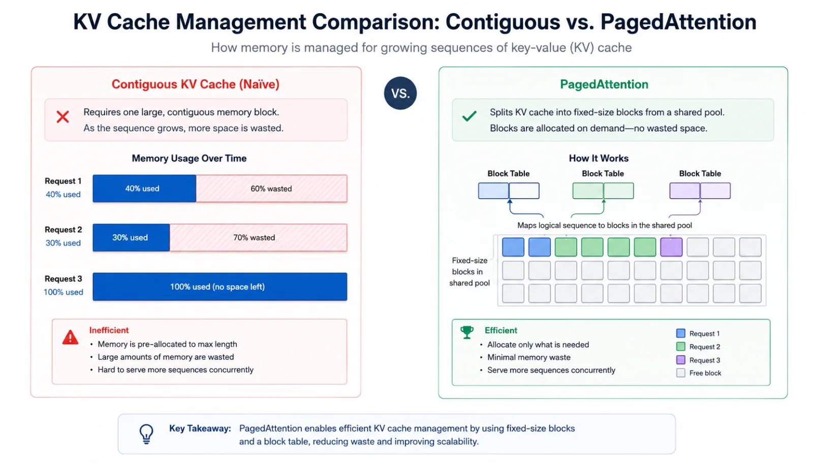Figure 5.0: Contiguous KV with wasted slots vs PagedAttention with a block table

8.4 Shrinking the cache itself

PagedAttention reclaims waste. Orthogonal architectural choices reduce the cache size to begin with:

Technique	Shrink	Quality cost	Stage
MHA — Multi-Head Attention (baseline)	1×	—	Pretrain
MQA — Multi-Query Attention (Shazeer 2019)	$H_q$×	small	Pretrain — PaLM, Falcon
GQA — Grouped-Query Attention (Ainslie 2023)	$H_q / g$×	~0	Pretrain — Llama 2/3, Mistral, Qwen
MLA (DeepSeek-V2/V3)	4–8× vs GQA	~0	Pretrain
FP8 KV	2×	~0	Inference (H100+)
INT4 KV (KIVI, KVQuant)	4×	small	Inference
Sliding window (Mistral 7B)	$S/W$×	medium	Pretrain
StreamingLLM (sinks + window)	$S/W$×	small	Inference
PagedAttention	reclaims waste	0	Inference

These stack. GQA + FP8 KV = 16× smaller than MHA BF16, no quality loss. Add PagedAttention and the remaining fragmentation is gone.

8.5 Throughput techniques

Throughput optimization splits into three families: attention kernels, batching policies, decoding strategies. Flash Attention, continuous batching, and speculative decoding are the headline members of each — useful to know as defaults, but each has siblings that win in specific regimes.

Attention kernels. Flash Attention (Dao et al. 2022) tiles $QK^T$ so $Q$, $K$, $V$ blocks stay in on-chip SRAM and the full $S \times S$ matrix is never materialized in HBM. Online softmax keeps numerics correct. Memory $O(N^2) \to O(N)$, wall-clock 2–4× faster. FA2 improved sequence-dim parallelism, FA3 added FP8 on Hopper at ~75% MFU. PyTorch’s F.scaled_dot_product_attention dispatches to one of these automatically — but the kernel space is wider than just FA:

Kernel	Specialty	Picked when
FlashAttention v1/2/3	tiled exact attention	default for training and prefill
xFormers `memory_efficient`	exact attention with custom masks	unusual masking patterns
FlexAttention (PyTorch 2.5+)	programmable mask/score function	one kernel, arbitrary attention pattern
FlashDecoding / FlashDecoding++	decode (small $Q$, long $K$)	KV long, batch small — SMs idle otherwise
FlashInfer	serving-templated CUDA kernels	TensorRT-LLM, SGLang, MLC backends
Ring Attention	sequence parallelism, exact	1M+ token contexts split across devices
Sliding window / sparse	structured sparsity (BigBird, SWA)	very long context, quality budget

Batching policies. Static batching waits until a full batch arrives, then processes all requests together — short requests wait for the longest to finish. Continuous (in-flight) batching (Orca 2022, used by vLLM, TGI, TensorRT-LLM) changes the batch composition at each decode step — finished requests free their slot immediately, queued requests join the batch mid-generation. 5–10× throughput improvement at typical workloads. The family:

Chunked prefill (Sarathi 2023) — splits long prefills into ~512-token chunks interleaved with decode, smoother TPOT under load at small TTFT cost.
Dynamic SplitFuse (DeepSpeed-FastGen) — fuses chunked prefills with decodes inside a single forward pass.
Disaggregated / Splitwise serving — run prefill on one GPU pool, decode on another, since the two phases have opposite compute/memory profiles.

Decoding strategies. Speculative decoding (Leviathan et al. 2022) has a small draft model emit $n$ candidate tokens, the target scores them in one forward pass, matches accept, mismatches restart drafting. Acceptance 60–80% → 2–3× speedup, distribution mathematically identical. The family:

EAGLE / EAGLE-2 / EAGLE-3 — fold drafting into a lightweight head on the target’s hidden states; no separate draft network.
Medusa — multiple parallel prediction heads forecasting at offsets $+1, +2, \ldots$
Lookahead decoding — algorithmic, no auxiliary model; Jacobi iteration on a sliding window.
Prompt lookup — for tasks with input-output overlap (code edits, RAG quoting), draft tokens come from the prompt itself.

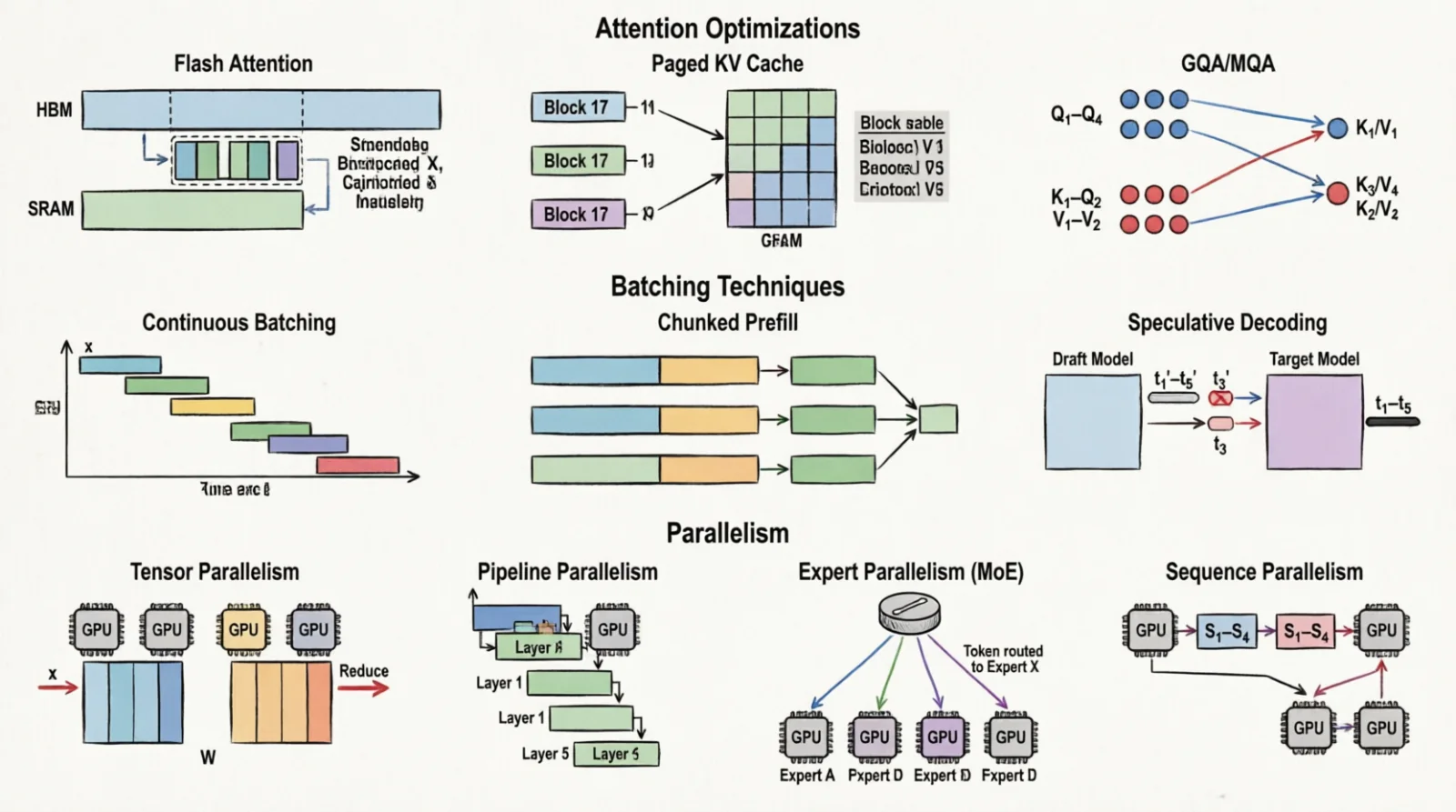Figure 6.0: Three families of throughput technique

8.6 Multi-GPU parallelism

When the model exceeds one GPU:

Strategy	What it splits	Communication	Best at
Tensor (TP)	Each layer’s matrices across GPUs (e.g., split weight matrix columns)	All-reduce (sum partial results from all GPUs, broadcast result back) after each layer	Intra-node, NVLink
Pipeline (PP)	Layers across GPUs (e.g., GPU0 gets layers 0-10, GPU1 gets 11-20)	Activations between stages	Cross-node, slower link
Expert (EP)	MoE experts	All-to-all dispatch (route tokens to expert GPUs)	MoE inference
Sequence (SP)	Activations along seq dim	Complements TP	Long context

Rule of thumb for Llama-405B serving: TP within a node (NVLink, 8 GPUs), PP across nodes (InfiniBand). For MoE: TP + EP.

8.7 Graph IRs and ahead-of-time compilers

Eager PyTorch executes ops one at a time. Each kernel writes its output to HBM and the next reads it back. To do better, the model has to be captured into a graph, optimized as a whole, and lowered to a backend that emits fused kernels. ONNX is one such graph format. It is not the only one — and the choice of IR (intermediate representation: a data structure representing the computation between source framework and target hardware) is often what determines the speedup ceiling.

Why graph-level optimization matters at all. The optimizer applies whole-graph transforms that eager mode cannot:

Constant folding — fold weights through frozen ops. Batch-norm absorbs into the preceding Conv; LayerNorm scales merge into the next matmul.
Operator fusion — Conv + BN + ReLU → one kernel; MatMul + Add + GELU → one fused matmul. The intermediate activations never leave registers.
Dead-code elimination — drop subgraphs whose outputs go unused (common after exporting only the inference path of a training model).
Shape specialization — when shapes are known, swap dynamic-shape kernels for static ones, unlocking pre-tuned code paths.
Algebraic simplification — collapse identity matmuls, fuse adjacent linear layers, hoist reshapes.

The FLOPs angle. Fusion barely changes the raw FLOP count. What changes is how many bytes those FLOPs cost. Conv + BN + ReLU as three kernels writes the activation to HBM, reads it back, writes it again — three round-trips. Fused, the activation lives in registers and shared memory; only the final output hits HBM. Same FLOPs, a fraction of the bytes, so arithmetic intensity rises and the workload moves up the roofline. A kernel that was memory-bound at intensity 50 may now sit at 200, compute-bound, with realized throughput 2–3× higher despite identical arithmetic.

The compiler landscape. Different IRs come with different backends, different fusion strategies, different sweet spots. The honest answer to “which one should I use” is “depends on the model, the hardware, and how much shape dynamism you need”:

Stack	IR	Strengths	Sweet spot
ONNX + ONNX Runtime	ONNX	broadest framework / hardware support	vision, encoders, multi-vendor deployment
TensorRT / TensorRT-LLM	proprietary (ONNX-importable)	most aggressive NVIDIA fusion	NVIDIA-only production inference
XLA + StableHLO	HLO / StableHLO (versioned HLO IR)	tracing JIT, TPU-first	JAX, TPU, large fused graphs
Apache TVM / MLC LLM	TIR, Relax	autoTVM / Ansor schedule search	edge, heterogeneous, mobile LLM
IREE	MLIR / Linalg	open MLIR stack, multi-backend	research, custom hardware, edge
`torch.compile` (Inductor)	FX → Triton DSL	in-process, no export step	PyTorch training and prototyping
TorchScript / `torch.export`	TS / EXIR	legacy / mobile-targeting PyTorch	older deployments, mobile via ExecuTorch
llama.cpp / GGUF	GGUF format (GPT-Generated Unified Format, model container)	CPU-first, aggressive quantization	local LLM on consumer hardware
OpenVINO	OV IR	Intel-tuned, CPU/iGPU/NPU	edge CPU inference

A few rules of thumb that follow:

If the model is a CNN or encoder and the deployment target varies (NVIDIA + Intel + ARM + mobile), ONNX + ORT with per-device execution providers is the path of least resistance.
If the target is fixed NVIDIA and you need the last 20% of throughput, TensorRT (for vision / generic) or TensorRT-LLM (for LLMs) beats ORT — at the cost of being NVIDIA-only and rebuilding the engine per shape regime.
If the workload is an LLM, none of the general-purpose graph compilers match a serving engine. vLLM, SGLang, and TensorRT-LLM beat ORT because PagedAttention, continuous batching, and KV-cache management are runtime concerns the ONNX graph abstraction has no way to express.
If you are still training and want fusion without an export step, torch.compile is the answer — Inductor generates Triton kernels on the fly and caches them.
If the model has to run on a laptop or phone, llama.cpp/GGUF or ExecuTorch matter more than the rest.

ONNX specifically. Once a model is exported (torch.onnx.export, TensorFlow tf2onnx, JAX → StableHLO → ONNX), the graph is detached from its source framework. ONNX Runtime executes it through execution providers — pluggable backends that translate ONNX ops to device-specific kernels, one per device class:

EP	Hardware	Notes
CUDA EP	NVIDIA	cuDNN/cuBLAS, baseline
TensorRT EP	NVIDIA	rebuilds the graph as a TensorRT engine, fastest for fixed shapes
ROCm EP / MIGraphX	AMD	parallel to TRT
OpenVINO EP	Intel CPU / iGPU / NPU	best CPU inference, INT8 calibration
CoreML EP	Apple	Neural Engine + GPU
QNN EP	Qualcomm Hexagon NPU	mobile / edge

  
import onnxruntime as ort

sess = ort.InferenceSession(
    "model.onnx",
    providers=[
        ("TensorrtExecutionProvider", {"trt_fp16_enable": True}),
        "CUDAExecutionProvider",      # fallback
        "CPUExecutionProvider",
    ],
)
out = sess.run(None, {"input": x})

Typical wins for vision and small encoder models: ORT + TensorRT EP gives 2–5× over eager PyTorch, mostly from fusion plus INT8/FP16 calibration. The ceiling is the same whether you got there through ONNX, TVM, or torch.compile — what differs is portability, dynamism tolerance, and how much hand-tuning the path requires.

Quantization. The other lever on realized FLOPs is dropping their precision: INT8 instead of FP16, INT4 weights with FP16 activations, FP8 end-to-end on Hopper. Hardware throughput more ops per cycle at lower precision (an H100 does 2× FP8 vs FP16), and weight reads from HBM shrink by the same ratio, which is the larger win for decode. All of the compilers above support some flavor of quantization — but the calibration mechanics (measuring activation distributions on representative data to set scaling factors), the algorithm choices (GPTQ, AWQ, SmoothQuant, QAT [quantization-aware training] vs PTQ [post-training quantization]), and the KV-cache variants get their own post next.

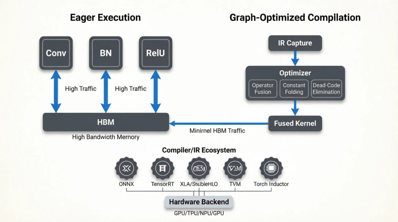Figure 7.0: From framework to device — IRs in the middle, backends on the right

8.8 Serving runtimes — vLLM, TIS, Ray Serve

vLLM is the open-source inference engine that built PagedAttention. Single command, OpenAI-compatible API, continuous batching, prefix caching:

  
python -m vllm.entrypoints.openai.api_server \
  --model meta-llama/Llama-3.1-70B-Instruct \
  --tensor-parallel-size 4 \
  --max-model-len 32768 \
  --kv-cache-dtype fp8

NVIDIA Triton Inference Server (TIS) — the runtime, distinct from Triton DSL. Loads multiple model formats (PyTorch, TensorRT, ONNX, OpenVINO, TF, vLLM-as-backend), batches requests dynamically, supports ensembles (model A → model B in one request), exposes HTTP/gRPC and Prometheus metrics. Where you go when you serve more than just LLMs:

name: "llama3_8b"
backend: "vllm"                          # vLLM-as-Triton-backend
max_batch_size: 32\text{VRAM} \approx \underbrace{N \cdot b_w}_{\text{weights}} + \underbrace{\text{kv}_{\text{tok}} \cdot S \cdot B}_{\text{KV cache}} + \underbrace{\text{activations}}_{\sim \text{small}} + \underbrace{\text{overhead}}_{1\text{-}2 \text{ GB}}
dynamic_batching {
  max_queue_delay_microseconds: 50000    # TTFT vs throughput knob
  preferred_batch_size: [ 8, 16 ]
}
instance_group [ { count: 1, kind: KIND_GPU } ]

Ray Serve sits above both. It does routing, model composition, autoscaling, and traffic splitting across deployments. Use it when you have many models, A/B tests, or pipelines (embed → rerank → LLM):

  
from ray import serve

@serve.deployment(num_replicas=2, ray_actor_options={"num_gpus": 1})
class LLMReplica:
    def __init__(self):
        from vllm import LLM
        self.engine = LLM(model="meta-llama/Llama-3.1-8B-Instruct")

    async def __call__(self, request):
        return self.engine.generate(request.prompt)

serve.run(LLMReplica.bind())

For training distribution, Ray Train wraps PyTorch DDP/FSDP with placement groups (a reservation of resources across the cluster that guarantees co-scheduling):

  
import ray
from ray.util.placement_group import placement_group

pg = placement_group([{"GPU": 2, "CPU": 16}] * 4, strategy="STRICT_SPREAD")

Each dict in the list is a “bundle” specifying resources. STRICT_SPREAD forces one bundle per node (spread across machines) — data parallelism across nodes. STRICT_PACK colocates everything on one node — tensor parallelism over NVLink. Get this wrong and you accidentally tensor-parallel over Ethernet, paying 100× latency on every layer.

For local heterogeneous inference (a Mac, a PC with a GPU, an iPhone all hosting one model), Exo splits the model by layer across devices. Throughput is bottlenecked by the slowest link, so it is for batch-1 personal use, not production.

8.9 KServe v2 plumbing

KServe is the Kubernetes-native serving CRD. An InferenceService resource wraps a model with autoscaling, traffic routing, and a standard request schema. Underneath it sits Knative (scale-to-zero, revisions) and Istio (routing, mTLS); the actual inference is delegated to a backend container — Triton, TorchServe, vLLM, MLServer, or a custom predictor.

The “v2” refers to the Open Inference Protocol (originally KFServing v2, now also implemented by Triton Inference Server, MLServer, TorchServe, and OpenVINO Model Server). One REST/gRPC contract, model-agnostic.

POST /v2/models/{name}/infer            # inference
GET  /v2/models/{name}                  # metadata
GET  /v2/models/{name}/ready            # per-model readiness
GET  /v2/health/ready                   # server liveness

The request body is a typed tensor list — same shape whether the backend is a ResNet on Triton or a Llama on vLLM:

  
{
  "inputs": [{
    "name": "input_ids",
    "shape": [1, 128],
    "datatype": "INT64",
    "data": [101, 2023, 2003, 1037, 3231, 102]
  }]
}

Responses mirror the same envelope under outputs. That uniformity is the point: a platform team (Seldon Core, BentoML, ModelMesh, KServe itself) can write one client and one observability pipeline regardless of which framework produced the model.

A minimal InferenceService wiring vLLM as the predictor:

  
apiVersion: serving.kserve.io/v1beta1
kind: InferenceService
metadata:
  name: llama3-8b
  annotations:
    serving.kserve.io/deploymentMode: RawDeployment # skip Knative for steady traffic
spec:
  predictor:
    minReplicas: 1
    maxReplicas: 8
    scaleTarget: 80 # target concurrency per replica
    containers:
      - name: kserve-container
        image: vllm/vllm-openai:latest
        args:
          - --model=meta-llama/Llama-3.1-8B-Instruct
          - --port=8080
        resources:
          limits:
            nvidia.com/gpu: "1"
        readinessProbe:
          httpGet: { path: /v2/health/ready, port: 8080 }

Three things this gives you that a raw vllm serve container does not:

Scale-to-zero via Knative. No traffic, the pods drain. The first request after idle pays a cold start (model reload, CUDA context, ~10–60 s for an 8B); subsequent requests are warm. Useful for long-tail models you cannot afford to keep resident.
Canary and traffic splitting. Two predictor revisions, 90/10 split, routed by the Istio virtual service KServe generates. Zero-downtime rollouts, automatic rollback on error rate.
Transformer and explainer pods. Pre/post-processing (tokenization, image decode, embedding lookup) runs in a transformer sidecar; explainability (SHAP, integrated gradients) runs in an explainer sidecar. The predictor stays focused on tensor math, which keeps GPU pods schedulable on GPU nodes and CPU pods on CPU nodes.

The hop count is the cost. A request flows: Istio gateway → Knative activator (only when scaled to zero) → queue-proxy sidecar → predictor container → backend engine. That is up to five hops before the model sees the input tensor. Each hop adds 1–5 ms. For LLM token streaming that is amortized across hundreds of tokens; for short classification calls it can dominate TTFT. Setting deploymentMode: RawDeployment skips Knative and drops two hops at the cost of losing scale-to-zero.

When KServe v2 earns its complexity: many models, mixed frameworks, autoscaling matters, you already run Kubernetes. When it does not: one model on one node — a bare vLLM container behind a load balancer is simpler, faster, and easier to reason about.

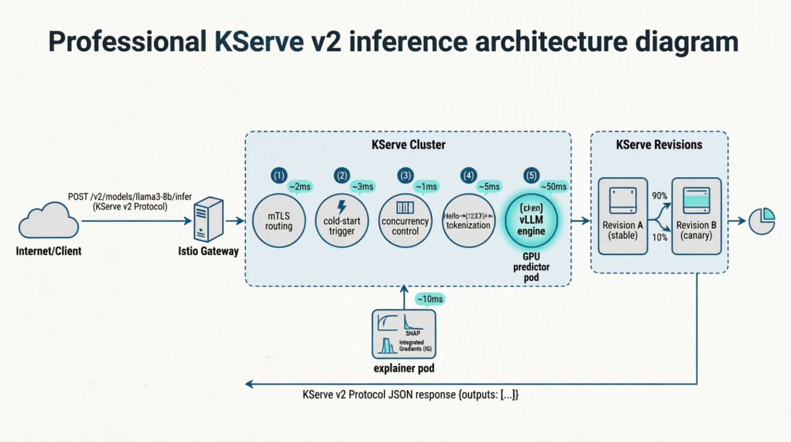Figure 8.0: A request through the KServe v2 stack — five hops before the model sees the tensor

8.10 Estimating VRAM for a model

\[\text{VRAM} \approx \underbrace{N \cdot b_w}_{\text{weights}} + \underbrace{\text{kv}_{\text{tok}} \cdot S \cdot B}_{\text{KV cache}} + \underbrace{\text{activations}}_{\sim \text{small}} + \underbrace{\text{overhead}}_{1\text{-}2 \text{ GB}}\]

For training, multiply weights by 4 (weights + gradients + Adam state). Llama-3 70B BF16 inference, 4K context, batch 1: 140 GB weights + 1.3 GB KV + ~3 GB activations + ~2 GB overhead = ~147 GB. Does not fit on H100 80 GB. Fits on H200 141 GB barely. Fits on 2× H100 with NVLink (160 GB).

9. The orchestration layer

§8 produced a serving process. §9 is what runs that process in production: a container, a scheduler that places it on a machine with the right hardware, and a way to give the container access to a GPU it doesn’t own.

The defaults are wrong for compute. Database containers are tuned for I/O — volume mounts, network latency, durable storage. Compute containers care about GPU access, shared-memory size, NUMA placement, and the inconvenient fact that the kernel driver they depend on lives on the host, outside the container’s filesystem.

9.1 The NVIDIA container stack

How does a container talk to a GPU whose driver lives on the host? It can’t ship the driver in the image (kernel code, bound to the host kernel version) — it bridges to the host driver at runtime. NVIDIA’s stack is a small tower:

GPU hardware
    ↓
NVIDIA kernel driver (host)
    ↓
libnvidia-container
    ↓
nvidia-container-toolkit / CDI
    ↓
Docker / containerd runtime
    ↓
Container (CUDA toolkit, cuDNN, PyTorch)

The split: driver and kernel module on the host; toolkit (userspace libs linking against the driver) inside the image. They meet at /dev/nvidia* nodes, injected into the container’s namespace (isolated view of system resources like filesystems, network, devices) at startup. The injection used to be a custom Docker runtime (--runtime=nvidia); the modern, runtime-agnostic mechanism is CDI (Container Device Interface), which containerd, Podman, and CRI-O all share.

  
nvidia-smi                          # host
nvidia-container-cli info           # toolkit
docker info | grep -i nvidia
docker run --rm --gpus all nvidia/cuda:12.4.0-base-ubuntu22.04 nvidia-smi
docker run --gpus '"device=0,1"' ...                # specific GPUs
docker run --gpus '"capabilities=compute,utility"' ...

9.2 BuildKit for ML images

ML images are large (5–15 GB) and rebuilt often. BuildKit (default builder since Docker 23.0) makes this bearable: cache mounts (pip/apt caches persist without ending up in the image), multi-stage builds (compile in one stage with full toolchain, copy artifacts to a slim runtime), multi-platform (AMD64 + ARM64 in one command), secret mounts (registry tokens without baking them in).

  
# syntax=docker/dockerfile:1.7
FROM nvidia/cuda:12.4.0-devel-ubuntu22.04 AS builder
RUN --mount=type=cache,target=/root/.cache/pip \
    --mount=type=cache,target=/var/cache/apt \
    apt-get update && apt-get install -y python3-pip && \
    pip install --prefix=/install torch==2.4.0 transformers vllm

FROM nvidia/cuda:12.4.0-runtime-ubuntu22.04
COPY --from=builder /install /usr/local
COPY app/ /app
WORKDIR /app
CMD ["python3", "-m", "vllm.entrypoints.openai.api_server", \
     "--model", "meta-llama/Llama-3.1-8B-Instruct"]

  
docker buildx build \
  --platform linux/amd64,linux/arm64 \
  --cache-to type=registry,ref=myregistry/vllm:cache,mode=max \
  --cache-from type=registry,ref=myregistry/vllm:cache \
  -t myregistry/vllm:latest --push .

9.3 Compose deploy with resources

docker-compose deploy.resources is the declarative way to pin GPU, CPU and memory. The compute-vs-IO distinction shows up in which fields matter:

  
services:
  inference:
    image: myregistry/vllm:latest
    shm_size: "16gb" # PyTorch DataLoader, NCCL
    ulimits:
      memlock: -1 # NCCL/CUDA pinning
      stack: 67108864
    deploy:
      resources:
        reservations:
          devices:
            - driver: nvidia
              device_ids: ["0", "1"] # specific GPUs (topology-aware)
              capabilities: [gpu]
          memory: 64G
          cpus: "16"
        limits:
          memory: 128G
    environment:
      - NCCL_DEBUG=INFO
      - CUDA_VISIBLE_DEVICES=0,1
      - PYTORCH_CUDA_ALLOC_CONF=expandable_segments:True

Three settings that catch people:

shm_size — Docker defaults to 64 MB of /dev/shm (shared memory: a tmpfs mounted in RAM, visible to all processes in the container, used for fast IPC). DataLoader workers use it to pass batches between processes; NCCL uses it for intra-node GPU communication. 64 MB is too small for ML workloads; set 4–16 GB.
ulimits.memlock: -1 — memlock (memory lock) is the limit on how much RAM a process can pin (prevent from being swapped to disk). NCCL and CUDA need to pin pages for RDMA and GPU DMA transfers. Default ulimit is often 64 KB, which blocks this. -1 means unlimited.
device_ids vs count — count: 2 says “any 2 GPUs”; device_ids: ['0','1'] says “specifically GPU 0 and 1”. The latter is what you want when NVLink topology matters (you need GPUs that are physically connected).

Setting	Compute-intensive	I/O-intensive
`deploy.resources.devices`	GPUs, MIG slices	Usually nothing
`shm_size`	4–16 GB	Default fine
`ulimits.memlock`	`-1`	Default
`cpus`	Pin to NUMA-local cores	Spread across cores
Volume mounts	Models (read-only, large)	Hot data (write, fsync)
Network	Intra-node mostly	Cross-node primary

For a compute job the Docker bridge often matters less than expected — most traffic is intra-node over NVLink. When it does matter (multi-node training, distributed inference), bypass it with network_mode: host or a CNI (Container Network Interface) plugin exposing RDMA (Remote Direct Memory Access: network protocol that allows direct memory-to-memory transfers between machines without CPU involvement) / InfiniBand.

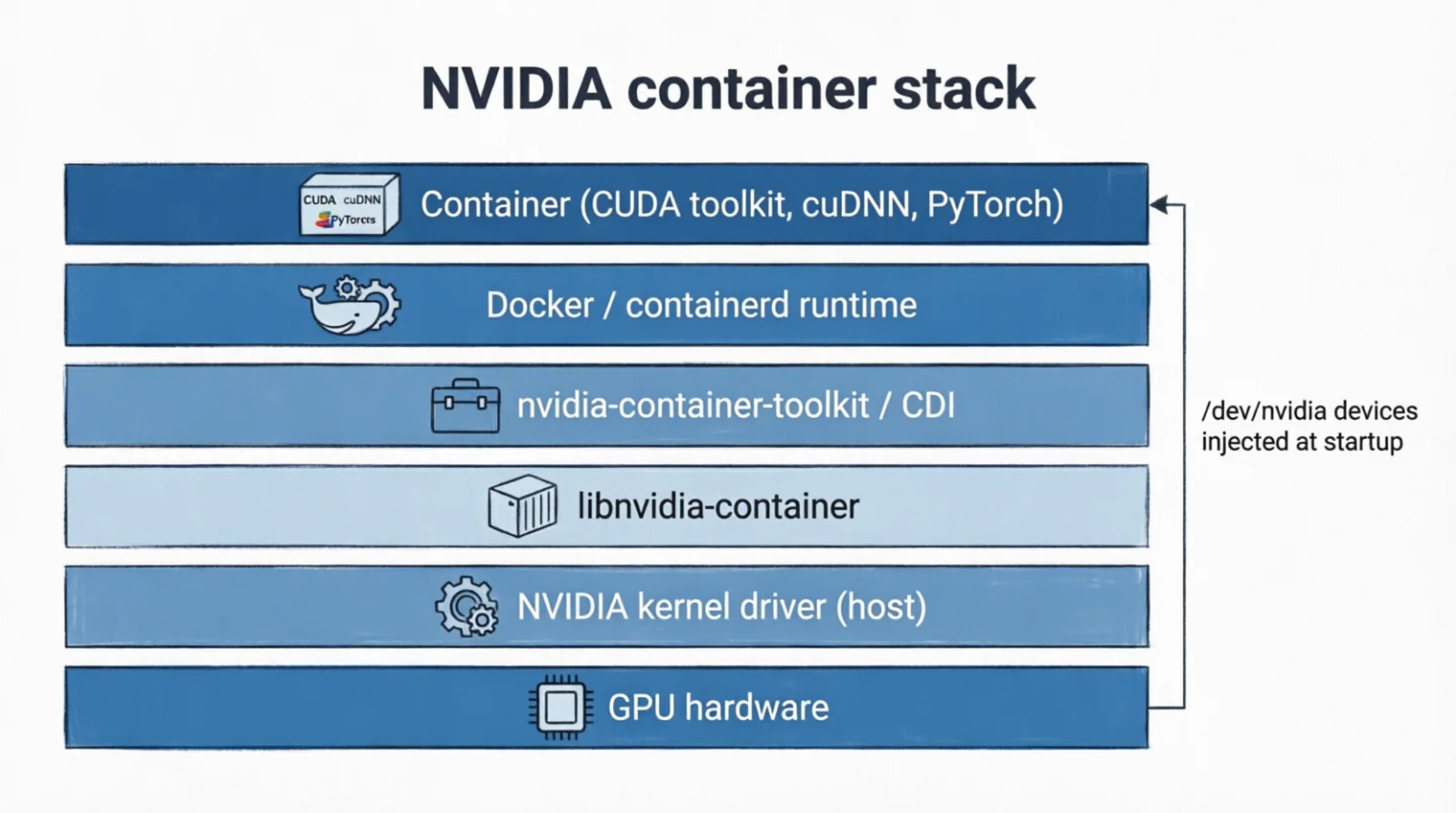Figure 9.0: Host driver, runtime, toolkit, container

10. Debugging order

When a compute workload is slow or broken, the layers to check, in order, because each layer assumes the ones below it work:

Kernel/driver/device. nvidia-smi, dmesg | grep -i xid. If the GPU is missing or throwing Xids, nothing above matters.
PCIe link. lspci -vvv | grep -E 'LnkCap|LnkSta'. Expected x16 Gen5, or did the BIOS downgrade it?
Topology. nvidia-smi topo -m, lstopo. Are the right GPUs on NVLink for your TP shards? Are loader threads on the right NUMA node?
Compiler/runtime. Driver CUDA version ≥ toolkit. Is torch.compile actually caching? ~/.cache/torch/inductor.
Math libraries. NCCL_DEBUG=INFO — are collectives over NVLink or falling back to TCP? cuDNN heuristics caching on stable shapes?
Allocator. torch.cuda.memory_summary(). Fragmenting? Set PYTORCH_CUDA_ALLOC_CONF=expandable_segments:True.
Framework. MFU below 30% on a compute-bound job means kernels are wrong (wrong dtype, wrong layout, no Tensor Core usage).
Serving. Flash Attention active? Continuous batching on? Prefix caching enabled?
Orchestration. shm_size, memlock ulimit, GPU device pinning, network mode for distributed.

Tuning kernels on a GPU that is silently in PCIe x4 mode is wasted effort. Walk bottom-up.

References

Systems & Infrastructure, ML Infrastructure

This post is licensed under CC BY 4.0 by the author.