Computer Vision Essentials

Primitive operations used across computer vision pipelines, and where they come from

Posted May 15, 2026 Updated May 16, 2026

By ibrahim_lahlou

20 min read

Computer Vision Essentials

Overview

The previous post covered convolution as one operation inside a CNN. This post stays at that level — individual operations — but widens the scope to the rest of the pipeline: how an image is represented, measured, transformed, normalized, and how its output is cleaned up.

A lot of these operations are older than deep learning. Histogram equalization comes from darkroom photography. Gamma correction comes from CRT physics. Non-maximum suppression comes from edge detection in the 80s. The neural-network era inherited them, gave a few of them learnable parameters, and added new ones on top. So for each one it helps to know not just the formula but where it came from and what problem the original author was trying to solve.

1. Image Representation

A digital image is a tensor $I \in \mathbb{R}^{H \times W \times C}$:

$H$: height (rows)
$W$: width (columns)
$C$: channels (3 for RGB, 1 for grayscale)

Pixel values are stored as uint8 in $[0, 255]$ or as float32 in $[0, 1]$ after scaling.

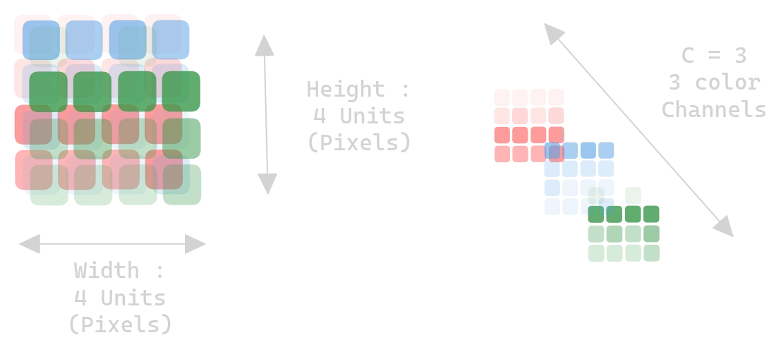
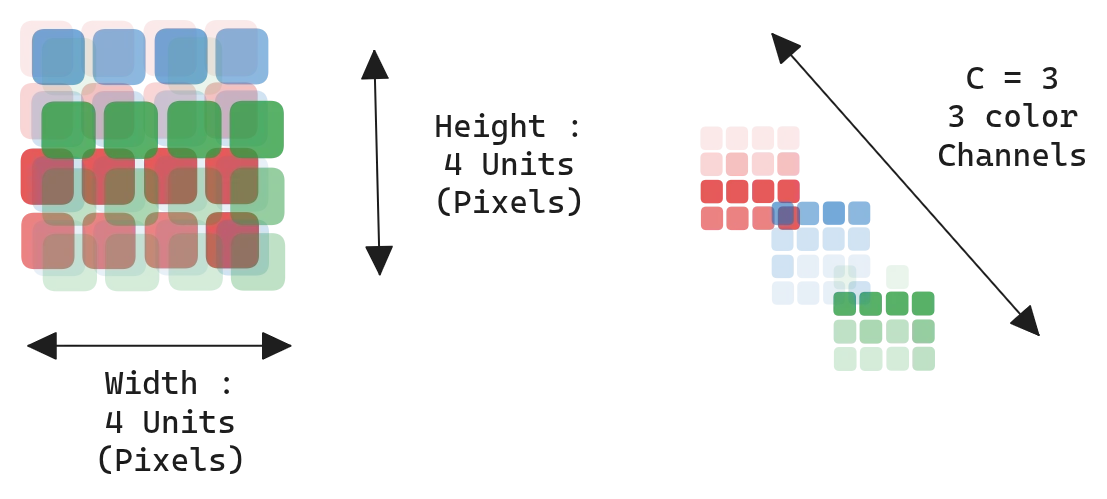Figure 1.0: An image as an H × W × C tensor

Color spaces

RGB is what a camera sensor produces and what a display consumes, so it’s the default. The other spaces exist because RGB mixes brightness and color together, which is awkward for tasks where you only care about one of the two. HSV pulls hue out as a separate channel — useful when you want to threshold on color. LAB tries to be perceptually uniform, meaning equal distances in LAB roughly correspond to equal perceived color differences. YUV separates luminance from chrominance and is what most video codecs operate on, because the human eye is less sensitive to chroma and you can compress it harder.

Space	Channels	Property
RGB	Red, Green, Blue	Additive, perceptually non-uniform
HSV	Hue, Saturation, Value	Decouples color from brightness
LAB	Lightness, A, B	Perceptually uniform
YUV	Luminance, Chrominance	Used in compression
Grayscale	Single intensity	No color information

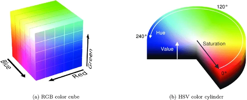Figure 2.0: RGB cube, HSV cylinder, LAB space

Normalization

Raw pixels in $[0, 255]$ have a mean around 100 and a large variance, which makes gradient descent slow and dependent on the initial learning rate. Standardizing per channel removes that:

\[\hat{x} = \frac{x - \mu}{\sigma}\]

with $\mu, \sigma$ computed on the training set. ImageNet uses $\mu = [0.485, 0.456, 0.406]$ and $\sigma = [0.229, 0.224, 0.225]$ — those constants got copied into nearly every codebase because so many models were pretrained on ImageNet.

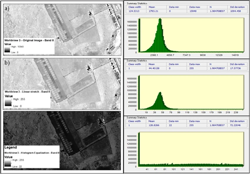Figure 3.0: Pixel distribution before and after standardization

2. Image Statistics

Before any modeling you usually want to know whether your images are even usable: too dark to see anything, distribution shift between train and test, color cast from a bad white balance. The operations in this section give you scalars you can threshold on. None of them are learned — they’re just descriptive statistics on a 2D array.

2.1 Contrast

Contrast is older than digital imaging. It’s how distinguishable a feature is from its surroundings, and it was studied by 19th and early-20th century vision scientists long before anyone applied it to a numpy array. There is no single formula because “how distinguishable” depends on what you’re looking at — a periodic grating, a small spot on a uniform background, or a natural photograph.

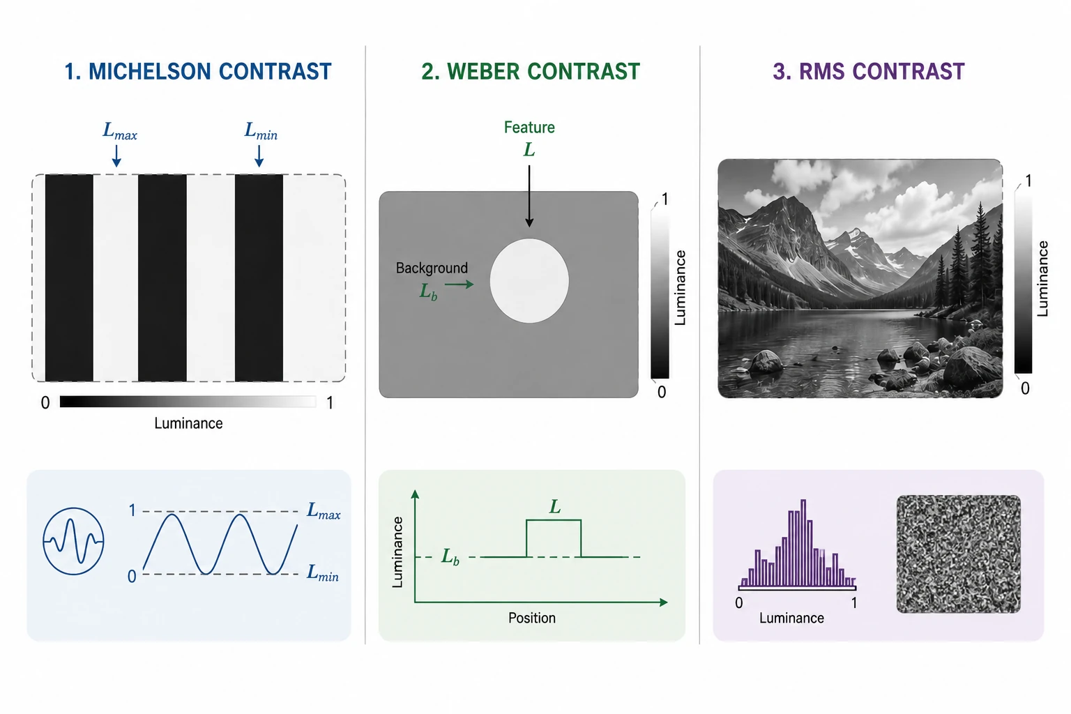Figure 4.0: Michelson, Weber, and RMS contrast

Michelson contrast came from Albert Michelson, the physicist who built optical interferometers and needed a number for how visible the resulting interference fringes were. The formula assumes a clean alternation between bright ($L_{max}$) and dark ($L_{min}$):

\[C_M = \frac{L_{max} - L_{min}}{L_{max} + L_{min}}\]

Weber contrast is older still — it comes out of Weber’s law (Ernst Weber, 1834), the empirical finding that the smallest change in luminance you can notice scales with the background luminance. So for a feature of luminance $L$ sitting on a background $L_b$, the relevant quantity is the ratio of the difference to the background:

\[C_W = \frac{L - L_b}{L_b}\]

RMS contrast is the one you actually compute on natural images, because they have no clean bright/dark or feature/background. It’s just the standard deviation of pixel intensity:

\[C_{RMS} = \sqrt{\frac{1}{HW}\sum_{i,j} (I[i,j] - \bar{I})^2}\]

RMS	Reading
< 10	Near-uniform
10 – 30	Low contrast
30 – 60	Normal
60 – 90	High
> 90	Hard clipping

2.2 Histogram statistics

A pixel-intensity histogram is the empirical distribution of brightness across the image. Treat it as a probability distribution and the usual statistical moments each say something different: the mean is exposure, the variance is contrast, the skew is how the distribution tilts (shadows-heavy or highlights-heavy), the kurtosis tells you about clipping at the extremes, and the entropy tells you how much information the image carries at all.

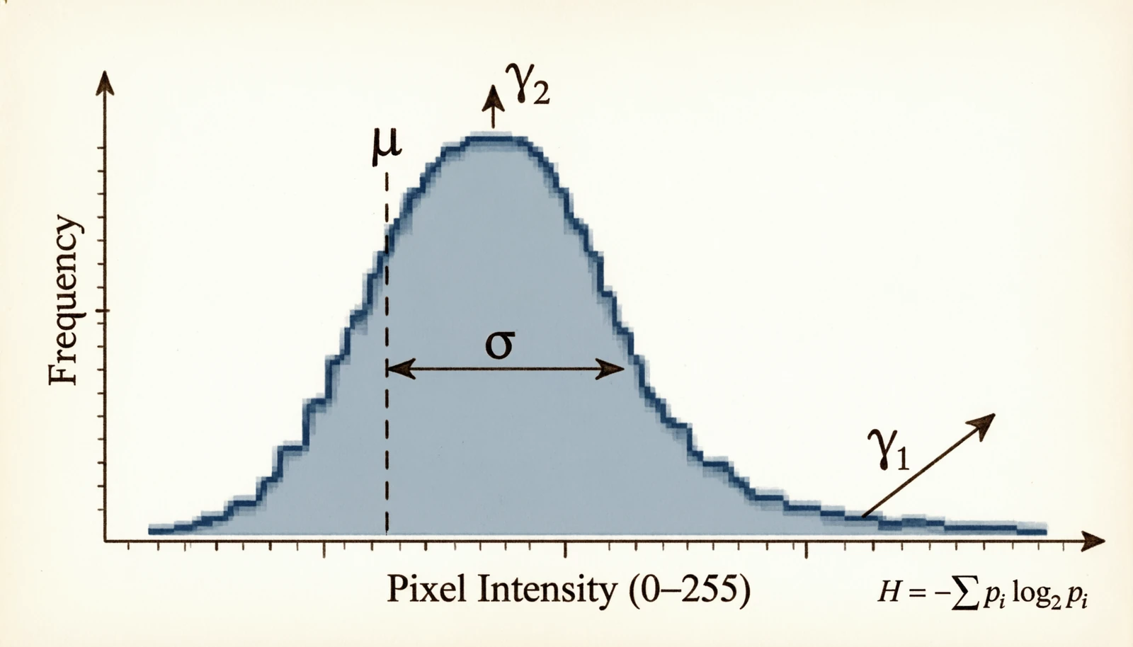Figure 5.0: Mean, variance, skew, kurtosis and entropy on a histogram

Let $p(k) = h(k)/(HW)$ be the normalized histogram.

\[\mu = \frac{1}{HW}\sum_{i,j} I[i,j], \quad \sigma^2 = \frac{1}{HW}\sum_{i,j} (I[i,j] - \mu)^2\] \[\gamma_1 = \frac{1}{HW \sigma^3}\sum_{i,j} (I[i,j] - \mu)^3 \quad (\text{skew})\] \[\gamma_2 = \frac{1}{HW \sigma^4}\sum_{i,j} (I[i,j] - \mu)^4 - 3 \quad (\text{kurtosis})\] \[H = -\sum_{k=0}^{255} p(k) \log_2 p(k) \quad (\text{entropy})\]

Metric	Value	Likely cause
$\mu$ < 50	Dark	Underexposed
$\mu$ > 200	Bright	Overexposed
$\sigma^2$ < 500	Flat	Low contrast
$\|\gamma_1\|$ > 1	Asymmetric	Gamma correction may help
$\gamma_2$ > 3	Heavy tails	Saturation, clipping
$H$ < 5 bits	Low info	Mostly uniform
$H$ > 7.5 bits	High info / noise	Worth a denoise check

2.3 Image-vs-image quality

These metrics exist because at some point you compare two images: a compressed version against the original, a denoiser’s output against the clean reference, a generated image against ground truth. The metrics got better as people noticed the older ones disagreed with human judgment.

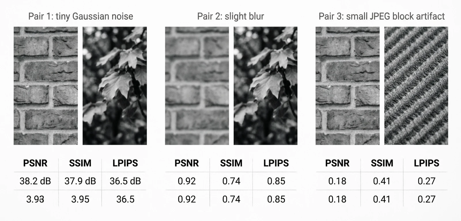Figure 6.0: PSNR, SSIM and LPIPS disagree on the same distortion

PSNR is the oldest. It came from analog signal transmission — a way to express how much noise a channel added to a signal. Adapted to images, it’s just pixel-level MSE on a logarithmic scale:

\[\text{PSNR} = 10 \log_{10}\!\left(\frac{\text{MAX}_I^2}{\text{MSE}}\right), \quad \text{MSE} = \frac{1}{HW}\sum (I_1 - I_2)^2\]

The problem with PSNR is that it weights every pixel difference equally. A small blur and a small amount of additive noise can have the same PSNR but look very different to a human — the blur is much less objectionable.

SSIM (Wang et al., 2004) was the response: instead of comparing pixel values directly, compare local luminance, contrast and structure separately.

\[\text{SSIM}(x, y) = \frac{(2\mu_x \mu_y + c_1)(2\sigma_{xy} + c_2)}{(\mu_x^2 + \mu_y^2 + c_1)(\sigma_x^2 + \sigma_y^2 + c_2)}\]

LPIPS (Zhang et al., 2018) went further. Rather than hand-design what “perceptually similar” means, take intermediate features from a network trained on ImageNet and compare those. It turns out those features align with human perception better than any handcrafted metric.

\[\text{LPIPS}(x, y) = \sum_l \frac{1}{H_l W_l}\sum_{h,w} \|w_l \odot (\phi_l(x)_{hw} - \phi_l(y)_{hw})\|_2^2\]

Metric	Good	Acceptable	Poor
PSNR (dB)	> 30	25 – 30	< 25
SSIM	> 0.85	0.70 – 0.85	< 0.70
LPIPS	< 0.15	0.15 – 0.30	> 0.30

2.4 Distribution comparison

These are classical statistical hypothesis tests, applied to image histograms instead of one-dimensional samples. The motivation is dataset shift: if the training and validation histograms disagree noticeably, the model is going to learn the training colors and exposure rather than the task.

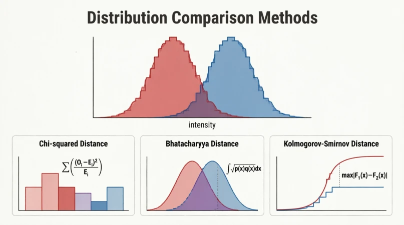Figure 7.0: χ², Bhattacharyya and KS on two overlapping histograms

\[\chi^2 = \sum_k \frac{(h_1(k) - h_2(k))^2}{h_1(k) + h_2(k) + \epsilon}\] \[D_B = -\ln\!\left(\sum_k \sqrt{p_1(k) p_2(k)}\right) \quad (\text{Bhattacharyya})\] \[D_{KS} = \max_k |F_1(k) - F_2(k)| \quad (\text{Kolmogorov-Smirnov})\]

A KS statistic above 0.2 between train and validation histograms usually means the splits are not from the same distribution.

2.5 Spatial autocorrelation

Moran’s I (Patrick Moran, 1950) was originally a spatial statistic for geography and ecology: do the values at neighboring locations tend to be similar (clustered) or dissimilar (dispersed)? The same scalar applies to pixels — it tells you whether the image has large smooth regions or fine alternating textures.

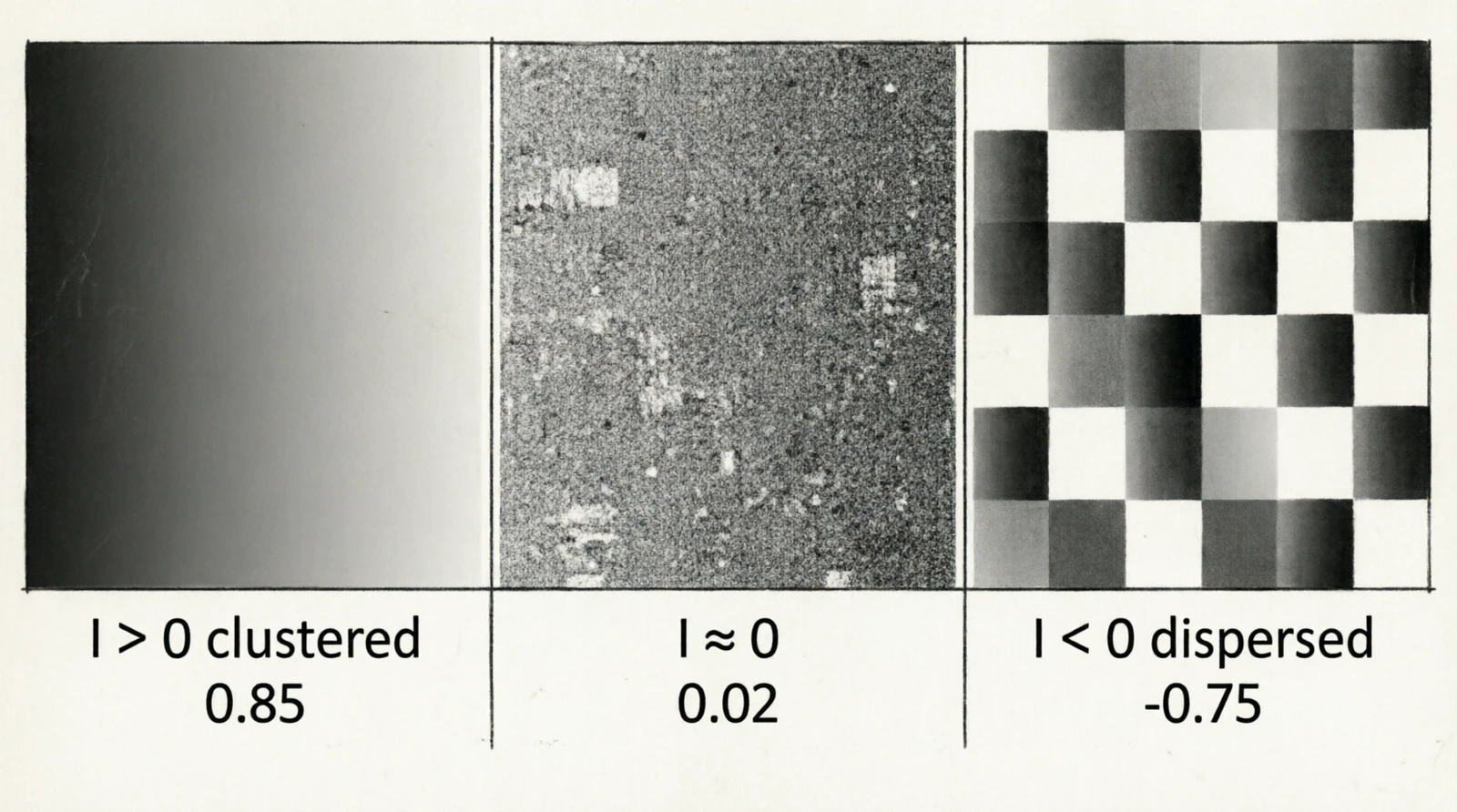Figure 8.0: Moran’s I on a smooth gradient, noise, and a checkerboard

\[R[u, v] = \sum_{i,j} I[i,j] \cdot I[i+u, j+v]\] \[I_M = \frac{N}{\sum_{i,j} w_{ij}} \cdot \frac{\sum_{i,j} w_{ij}(x_i - \bar{x})(x_j - \bar{x})}{\sum_i (x_i - \bar{x})^2}\]

$I_M > 0$ means clustered values (smooth regions), $I_M \approx 0$ is noise, $I_M < 0$ is alternating patterns like checkerboards.

3. Preprocessing

Deterministic transformations applied to the image before it enters the model. Most predate deep learning by decades and come from photography or signal processing.

3.1 Histogram equalization

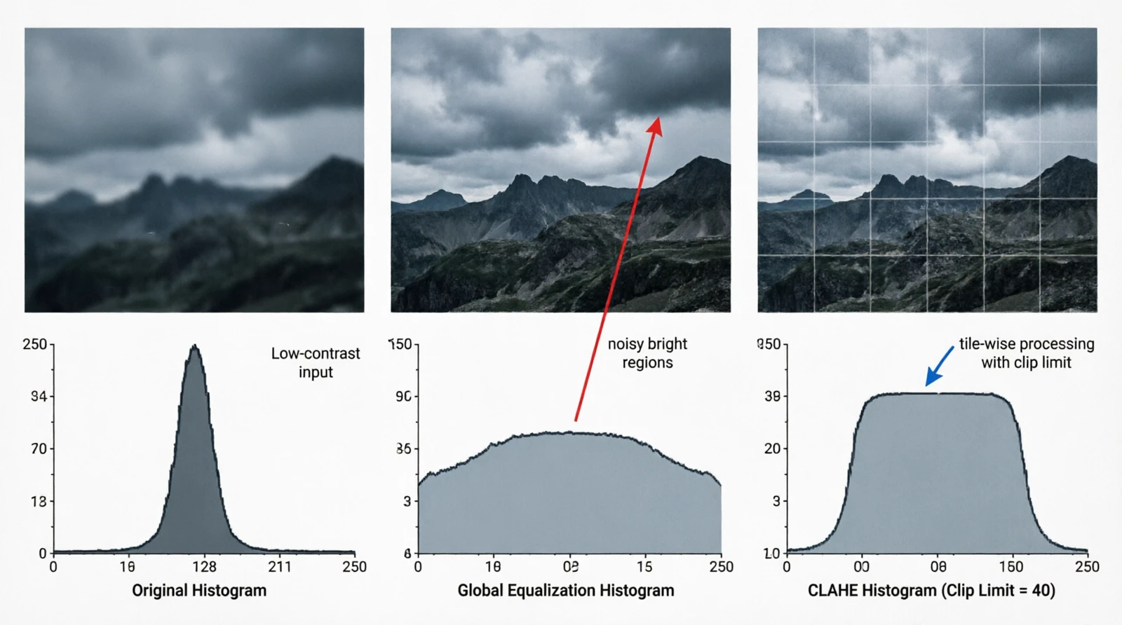
Figure 9.0: Global equalization vs CLAHE

This is a darkroom-era idea: if the brightness histogram is bunched in one part of the range, remap intensities so it spreads across the whole range. Formalized for digital images in the 70s. The map is the cumulative distribution scaled to the output range:

\[T(k) = \lfloor (L-1) \cdot \text{CDF}(k) \rfloor, \quad \text{CDF}(k) = \sum_{i=0}^{k} p(i)\]

Global equalization stretches contrast everywhere, including regions that already had plenty of it, which amplifies noise in bright areas. CLAHE (Pizer et al., 1987) was introduced for medical imaging where this was unacceptable: it splits the image into tiles and equalizes each one with a clipping limit on the histogram before integration.

  
import cv2
clahe = cv2.createCLAHE(clipLimit=2.0, tileGridSize=(8, 8))
out = clahe.apply(gray_image)

3.2 Gamma correction

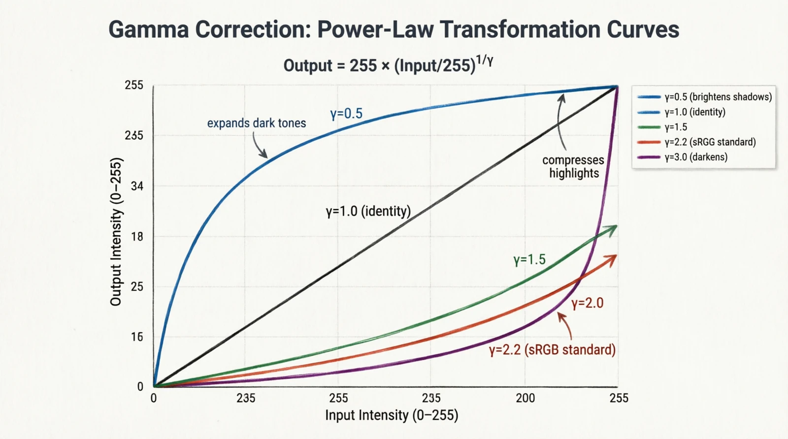Figure 10.0: Gamma curves for γ = 0.5, 1, 1.5, 2.2, 3

Gamma is a leftover from CRT displays. The brightness of a phosphor was a non-linear function of the input voltage, roughly $V^{2.2}$. Cameras applied the inverse curve when encoding the signal so that the display, by undoing it, produced a linearly correct image. The convention outlived the hardware: the sRGB color space encodes images with $\gamma \approx 2.2$, and “gamma correction” is the pointwise remap used to encode, decode, or deliberately brighten/darken:

\[I'[i,j] = 255 \cdot \left(\frac{I[i,j]}{255}\right)^\gamma\]

$\gamma < 1$ brightens shadows
$\gamma = 1$ is identity
$\gamma > 1$ darkens and compresses highlights
$\gamma = 2.2$ is the sRGB ↔ linear conversion

3.3 White balance

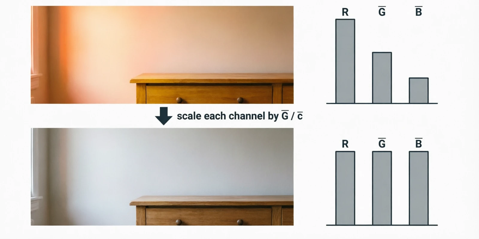Figure 11.0: Gray-world white balance before and after

Different light sources have different color temperatures — tungsten lamps are warm (~3200 K), midday daylight is cool (~6500 K) — and a sensor records the same scene differently under each. White balance is the correction. The simplest version is the gray-world assumption (Buchsbaum, 1980): averaged over a natural scene, the three channels should be roughly equal. If they’re not, scale each channel until they are.

A scalar measure of how far off we are:

\[\text{cast} = \frac{\max(\bar{R}, \bar{G}, \bar{B}) - \min(\bar{R}, \bar{G}, \bar{B})}{\bar{R} + \bar{G} + \bar{B}}\]

And the correction:

\[I'_c[i,j] = I_c[i,j] \cdot \frac{\bar{G}}{\bar{c}}, \quad c \in \{R, G, B\}\]

4. Feature extraction primitives

Three operation types make up almost every modern vision model. The previous post showed convolution. The story since then has been about how much non-locality the network is allowed to have, and how early.

4.1 Convolution (local)

A small kernel reused across every spatial location:

\[y[i,j] = \sum_{a,b} K[a,b] \cdot x[i+a, j+b]\]

Variants exist because the basic operation is expensive and people have found cheaper ways to approximate parts of it:

Variant	Receptive field	Parameters
Standard	$k \times k$	$k^2 C_{in} C_{out}$
Depthwise	$k \times k$ per channel	$k^2 C$
Pointwise (1×1)	$1 \times 1$	$C_{in} C_{out}$
Dilated	$k \times k$ with gaps	$k^2 C_{in} C_{out}$
Transposed	inverse mapping	$k^2 C_{in} C_{out}$

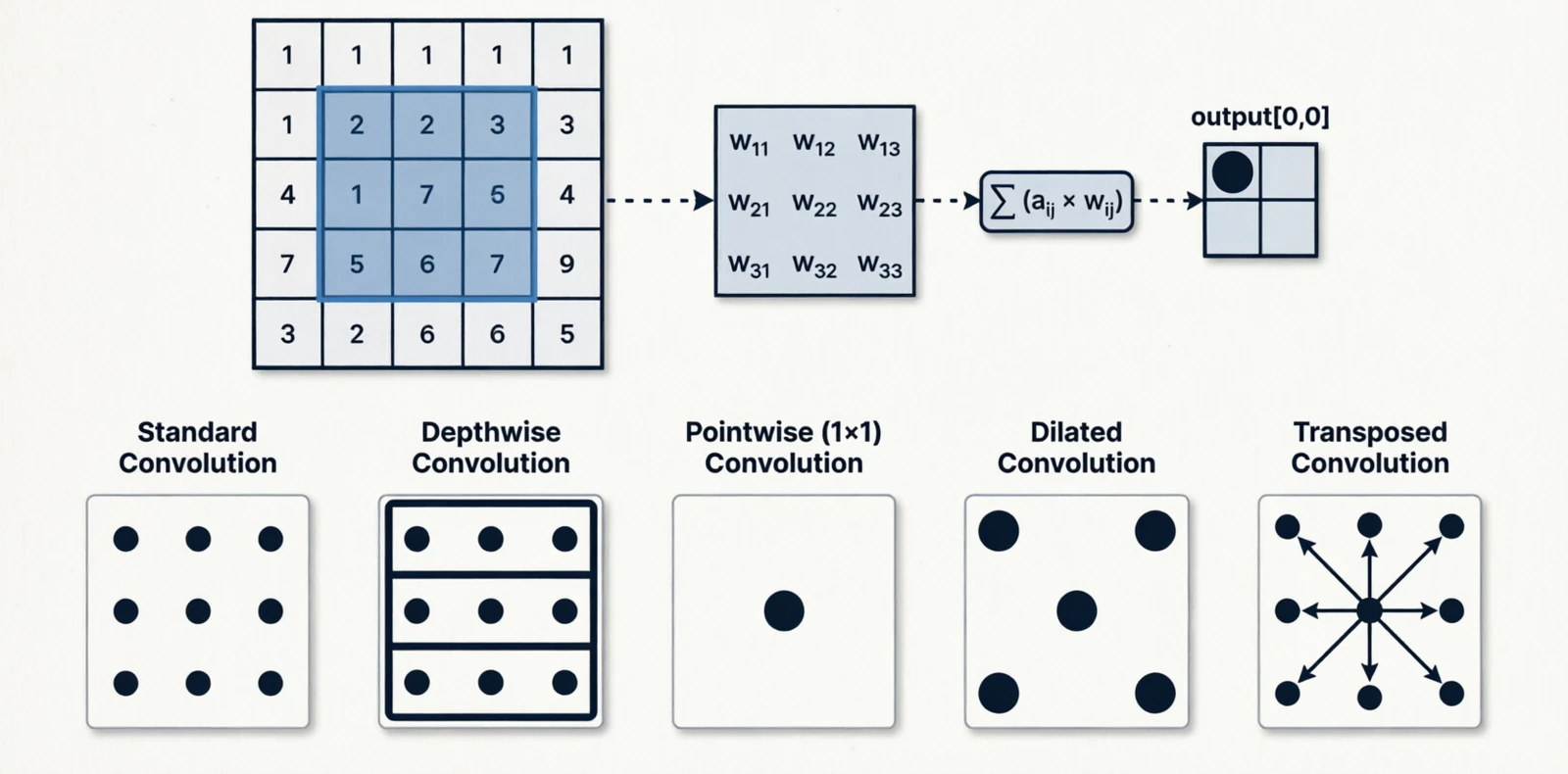Figure 12.0: Standard, depthwise, pointwise, dilated, and transposed convolution

4.2 Self-attention (global)

Attention came from machine translation (Bahdanau et al., 2014), where a decoder needed to look at a variable subset of the encoder’s outputs. It was generalized to self-attention in the Transformer (Vaswani et al., 2017), where every token in a sequence attends to every other token. The vision version is the same idea on image patches.

\[\text{Attn}(Q, K, V) = \text{softmax}\!\left(\frac{QK^T}{\sqrt{d_k}}\right)V\]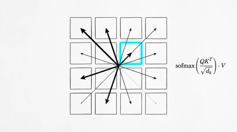

Figure 13.0: Self-attention on image patches

The trade-off against convolution is straightforward. Convolution has a strong prior — “pixels nearby in space are more related” — which is useful on small datasets but a constraint at scale. Self-attention has no such prior and has to learn relationships from data, which is what makes it data-hungry but very flexible.

	Convolution	Self-attention
Receptive field	Local, grows with depth	Global from layer 1
Cost	$O(HW \cdot k^2 C)$	$O((HW)^2 C)$
Inductive bias	Strong (locality)	Weak
Data efficiency	High	Lower, needs more pretraining

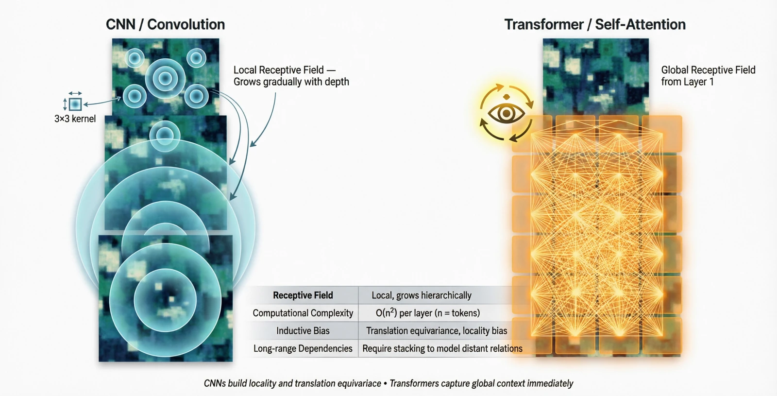Figure 14.0: Receptive field growth in CNN vs Transformer

4.3 Mixing the two

A common pattern is convolution in the early stages (cheap, local) and attention in the late stages (global reasoning on a smaller spatial grid). The early features are mostly about textures and edges, which are local anyway; by the late stages the spatial map is small enough that the $O((HW)^2)$ cost is no longer the bottleneck.

5. Spatial operations

Operations that change the resolution. Downsampling for efficiency and broader receptive field, upsampling when the task needs pixel-level outputs again.

5.1 Downsampling

Max pooling was introduced in the neocognitron (Fukushima, 1980), an early hierarchical model of the visual cortex. It was meant to mimic complex cells, which respond to a feature anywhere within a small region — the max being a soft form of “anywhere”. It became the default in early CNNs and remained so until strided convolution replaced it: a single learned filter that downsamples while extracting features, removing the need for a separate non-learnable layer.

Blur pooling (Zhang, 2019) revisited the question and pointed out something the field had ignored: naive subsampling violates the Nyquist criterion and causes aliasing, which is one reason CNNs are not truly shift-invariant. A small Gaussian blur before subsampling fixes it.

Method	Operation	Learnable
Max pooling	$\max$ over window	No
Average pooling	mean over window	No
Strided convolution	learned filter	Yes
Blur + subsample	Gaussian then stride	No

5.2 Upsampling

Transposed convolution learns to upsample, but it tends to produce checkerboard artifacts when stride and kernel size do not divide cleanly — this was diagnosed in detail by Odena et al. (2016). Pixel shuffle (also called sub-pixel convolution, Shi et al., 2016) avoids the artifact entirely: instead of inserting zeros and convolving, it convolves first to produce extra channels, then rearranges those channels into spatial positions.

Method	How	Notes
Nearest neighbor	repeat pixels	Blocky
Bilinear / bicubic	polynomial interpolation	Smooth
Transposed convolution	learned	Can produce checkerboard artifacts
Pixel shuffle	reshape channels into space	Same cost as conv, no checkerboard

5.3 Multi-scale combination

Detection has to handle objects from a few pixels to most of the image. The old approach was the image pyramid: resize the input to several scales and run the network on each, which was expensive. The Feature Pyramid Network (Lin et al., 2017) made the observation that the network itself already produces feature maps at different resolutions internally — the deeper ones are semantically rich but coarse, the shallower ones are spatially precise but semantically thin. Combining them top-down gives you the best of both at every scale:

\[P_l = \text{Conv}(C_l + \text{Upsample}(P_{l+1}))\]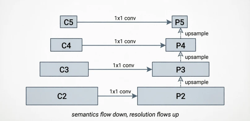

Figure 15.0: Bottom-up backbone with top-down pyramid

6. Channel operations

Operations on the channel axis decide which features get amplified or suppressed. The spatial axis tells you where something is; the channel axis tells you what it is.

6.1 1×1 convolution

Introduced as “network-in-network” (Lin et al., 2013) and popularized by Inception. It has no spatial reach — at each pixel, it is just a learned linear combination across channels:

\[y_c[i,j] = \sum_{c'} W[c, c'] \cdot x_{c'}[i,j]\]

The usual purpose is to change the channel count cheaply, either to compress before an expensive 3×3 convolution or to match dimensions for a residual connection.

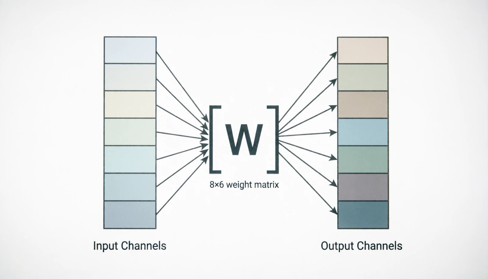Figure 16.0: 1×1 convolution as pure channel mixing

6.2 Channel attention

Squeeze-and-Excitation (Hu et al., 2018) added a tiny side branch that produces one weight per channel, computed from the global pooled features, and rescales the activations:

\[s_c = \sigma(W_2 \cdot \text{ReLU}(W_1 \cdot \text{GAP}(x_c))), \quad y_c = s_c \cdot x_c\]

Almost no extra cost, consistent accuracy gain; the original paper won the last ImageNet classification challenge.

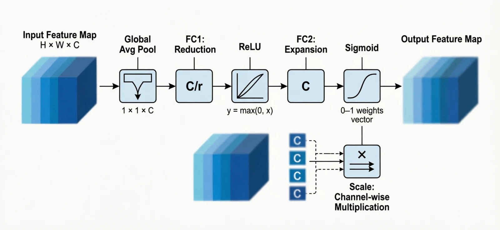Figure 17.0: Squeeze-and-Excitation block

6.3 Spatial attention

The dual of channel attention: pool over channels at each pixel, then learn a per-pixel weight. CBAM (Woo et al., 2018) chained channel attention with spatial attention in the same block.

\[s[i,j] = \sigma(\text{Conv}([\text{MaxPool}_{ch}(x), \text{AvgPool}_{ch}(x)]))\]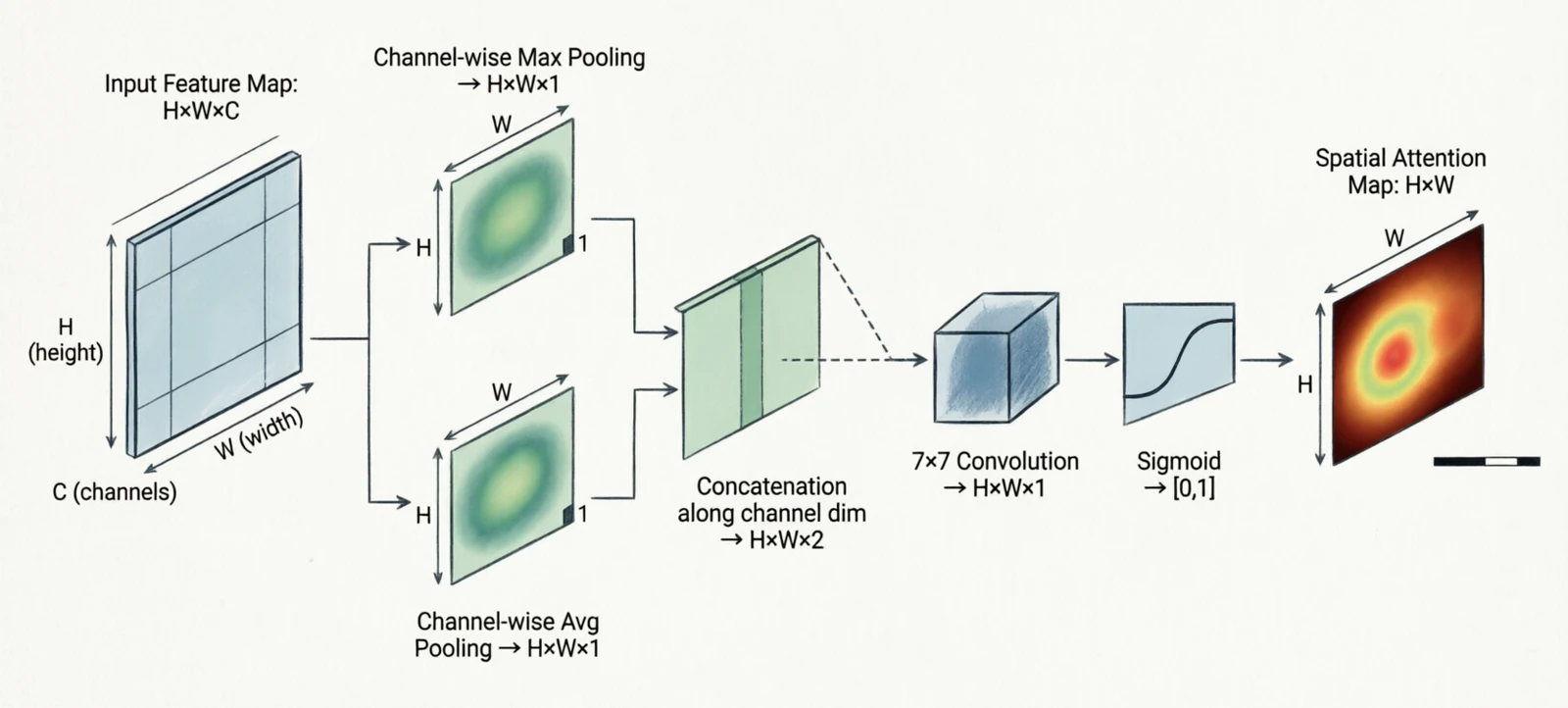

Figure 18.0: Channel + spatial attention (CBAM)

7. Normalization

BatchNorm (Ioffe & Szegedy, 2015) was the first normalization layer that made deep networks train reliably without careful initialization or low learning rates. The paper’s stated motivation — “internal covariate shift” — has since been disputed, and the actual reason it helps is still debated, but the empirical effect is real and the technique became standard in a year.

The variants that followed exist because BatchNorm’s statistics are computed across the batch, which breaks down when the batch is small (detection, segmentation, video) or when the model is recurrent. Each variant moves the reduction to different axes.

For activation tensor $x \in \mathbb{R}^{N \times C \times H \times W}$:

Variant	Reduces over	Depends on batch?	Why it was introduced
BatchNorm	$(N, H, W)$ per channel	Yes	Stable training in CNNs
LayerNorm	$(C, H, W)$ per sample	No	RNNs, transformers (no batch axis)
InstanceNorm	$(H, W)$ per channel per sample	No	Style transfer
GroupNorm	$(H, W, G)$ per group	No	Small batches in detection

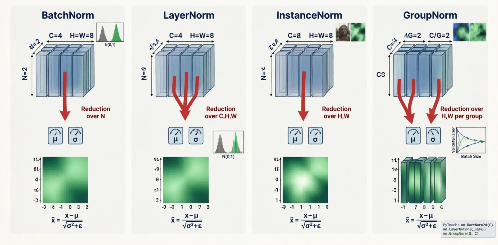Figure 19.0: BatchNorm, LayerNorm, InstanceNorm, GroupNorm — which axes each reduces over

A rough rule for picking one:

Batch size	Pick
1 – 4	LayerNorm or GroupNorm
8 – 16	GroupNorm
32+	BatchNorm

When fine-tuning a BatchNorm model on a small batch, freeze the running statistics rather than recomputing them.

8. Augmentation

Augmentation enlarges the effective training set by applying random transformations the model is supposed to be invariant to. Geometric and photometric augmentations are old and intuitive — a cat is still a cat after a horizontal flip or a brightness shift. The interesting category is the third one.

MixUp (Zhang et al., 2017) trains on linear interpolations of two samples and their labels. This seems wrong — a 50/50 blend of a cat and a dog is not a real image — but it works, partly because it pushes the model toward linear behavior between training examples, which smooths the decision boundary.

\[\text{MixUp:} \quad x' = \lambda x_i + (1-\lambda) x_j\]

CutMix (Yun et al., 2019) avoided MixUp’s unnatural blending by pasting a rectangular patch of one image onto another:

\[\text{CutMix:} \quad x' = M \odot x_i + (1 - M) \odot x_j\]

CutOut (DeVries & Taylor, 2017) is the same thing where the pasted region is zeros — it forces the model to look at other parts of the image rather than fixating on one discriminative region.

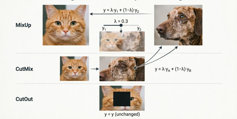Figure 20.0: MixUp, CutMix and CutOut

9. Losses

A loss is the contract between the model and the task. Three groups, depending on what the output looks like.

Pixel regression

L1 and L2 are the classical regression losses. Smooth L1 is the Huber loss (Huber, 1964) — L2 near zero, L1 in the tails — adopted in Fast R-CNN for bounding-box regression so that a single misaligned box would not blow up the gradient.

Loss	Formula	Behavior
L1	$\|y - \hat{y}\|$	Robust, sharp
L2	$(y - \hat{y})^2$	Smooth, sensitive to outliers
Smooth L1	hybrid	Robust + smooth
Charbonnier	$\sqrt{(y-\hat{y})^2 + \epsilon^2}$	Differentiable L1

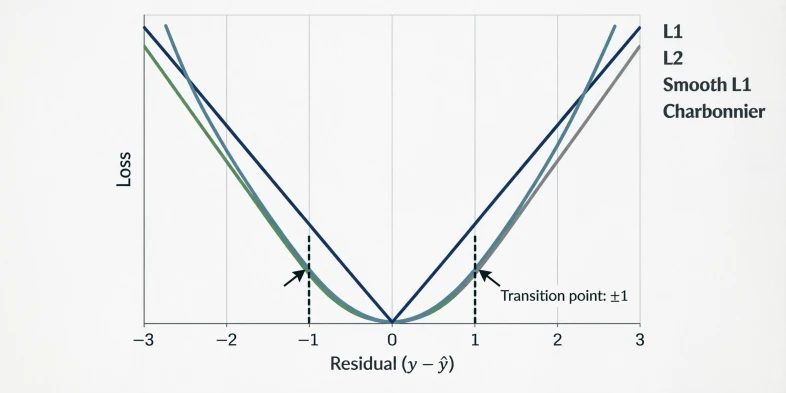Figure 21.0: L1, L2, Smooth L1 and Charbonnier curves

Classification

Plain cross-entropy is the default. Focal loss (Lin et al., 2017) was introduced for single-stage object detectors, where most candidate boxes are easy background and cross-entropy ends up dominated by those easy negatives. Multiplying CE by $(1 - p)^\gamma$ suppresses the contribution of confident predictions. Label smoothing addresses the opposite problem: hard one-hot targets push the model toward overconfidence, which hurts calibration; replacing them with $1 - \epsilon$ on the true class and $\epsilon / (K-1)$ elsewhere softens this.

Embedding losses

These exist because for tasks like face recognition you do not want a fixed number of classes — you want an embedding space where same-identity samples are close and different-identity samples are far. Triplet loss (FaceNet, Schroff et al., 2015) makes this explicit: an anchor, a positive (same class), and a negative (different class), with a margin. InfoNCE generalizes to many negatives at once and is the loss behind most self-supervised contrastive learning — treat augmentations of the same image as positives, everything else in the batch as negatives.

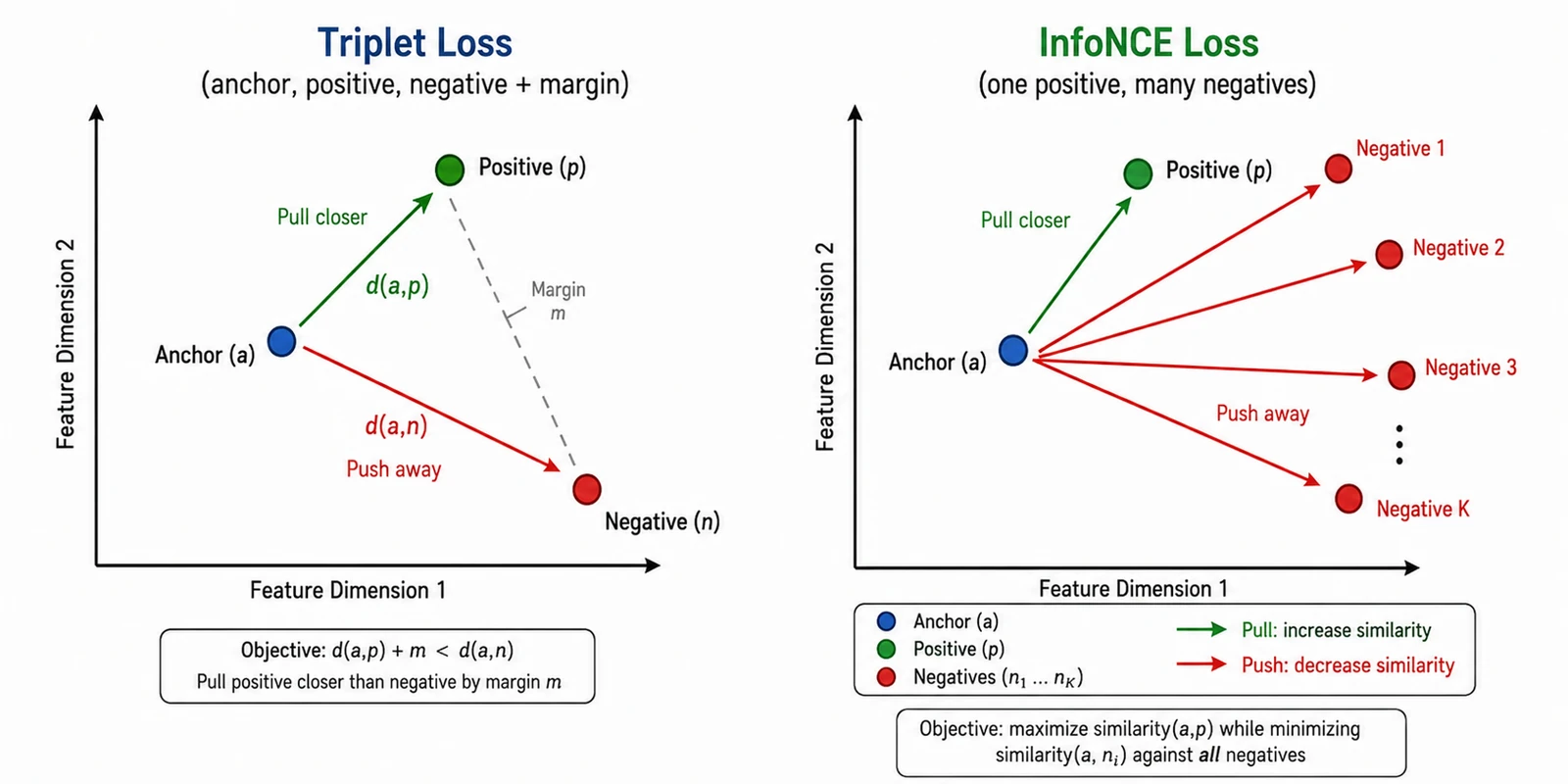Figure 22.0: Triplet and InfoNCE in embedding space

Multi-task

When the model has multiple heads:

\[L = \sum_i \lambda_i L_i\]

The weights $\lambda_i$ matter as much as the losses themselves, and tuning them is annoying enough that there are entire papers on automating it.

10. Postprocessing

After a model runs, the raw output is rarely what you ship.

10.1 Non-maximum suppression

The name comes from Canny edge detection (Canny, 1986), where pixels that were not the local maximum of the gradient magnitude along the edge direction were suppressed, leaving thin one-pixel edges. The detection-box version is the same idea on overlapping proposals: for each cluster of overlapping boxes, keep the one with the highest confidence and drop the rest if their overlap is high.

\[\text{IoU}(B_1, B_2) = \frac{|B_1 \cap B_2|}{|B_1 \cup B_2|}\]

Standard threshold $\tau = 0.5$. Soft-NMS (Bodla et al., 2017) was introduced for crowded scenes where two genuinely different objects can overlap significantly — instead of dropping the lower-confidence box, it decays its score:

\[s_i \leftarrow s_i \cdot e^{-\text{IoU}(M, B_i)^2 / \sigma}\]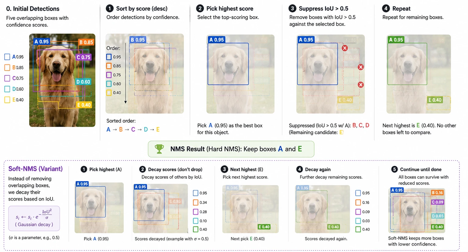

Figure 23.0: NMS and Soft-NMS on overlapping boxes

10.2 Temperature scaling

Guo et al. (2017) pointed out something that had been quietly true for a while: modern deep classifiers output probabilities that do not match their actual accuracy. A model that says “90% confident” might only be right 70% of the time. The fix is almost embarrassingly simple — divide the logits by a single scalar $T$ fit on the validation set:

\[p(c) = \frac{e^{z_c / T}}{\sum_{c'} e^{z_{c'} / T}}\]

$T > 1$ softens the distribution, $T < 1$ sharpens it. The metric you track is the expected calibration error:

\[\text{ECE} = \sum_m \frac{|B_m|}{N} |\text{acc}(B_m) - \text{conf}(B_m)|\]

ECE > 0.05 is usually worth correcting.

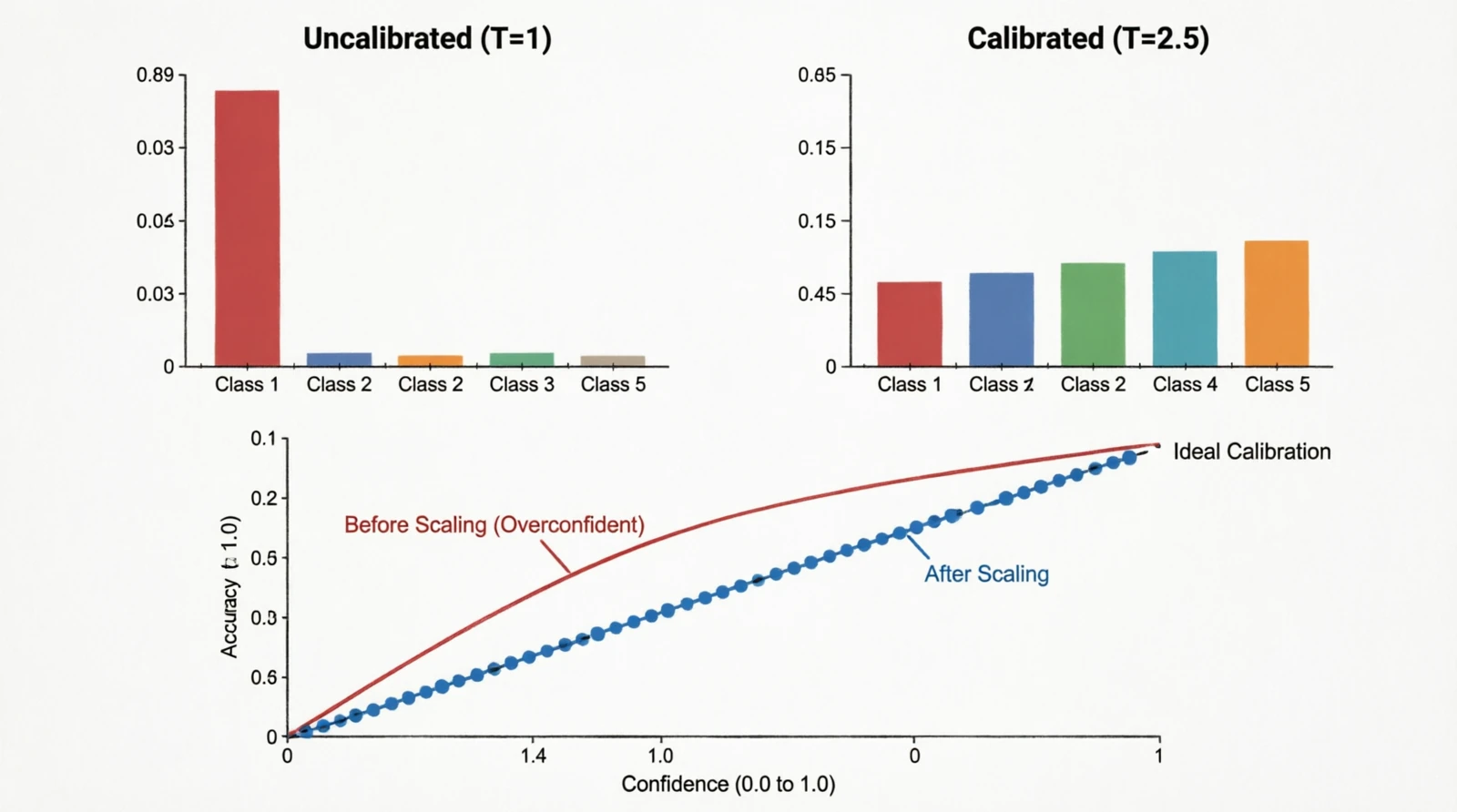Figure 24.0: Softmax distribution and reliability diagram before/after temperature scaling

References

Machine Learning, Computer Vision, Deep Learning

This post is licensed under CC BY 4.0 by the author.