Text operations in neural networks

Overview

Text operations in neural networks involve transforming text data into numerical representations that machines can process. These operations are fundamental to Natural Language Processing (NLP) tasks. The primary challenge is converting variable-length text sequences into fixed-size numerical representations while preserving semantic meaning and contextual relationships.

How Text Processing Works in Neural Networks:

Text processing typically follows a pipeline of operations: tokenization, embedding, and contextual encoding. Each step transforms the text into increasingly sophisticated representations that capture different aspects of language structure and meaning.

Why Use Text Operations?

• Numerical Representation: Neural networks can only process numerical data, requiring text to be converted into vectors or matrices.

• Semantic Preservation: Operations must maintain meaningful relationships between words and phrases while converting to numerical form.

• Context Handling: Text operations need to capture both local (nearby words) and global (document-level) context.

Text Operations

Tokenization

What is Tokenization?

Tokenization converts raw text into discrete token IDs that neural networks can process. The input is text; the output is integers representing semantic units.

Example:

Input: "The cat sat"
Tokens: ["The", "cat", "sat"]
Token IDs: [101, 2117, 2849]

The core question: What should count as a token? The answer determines downstream model performance.

Tokenization Granularity: Three Levels

1. Word-Level Tokenization

Split text by whitespace and punctuation. Each word becomes a token.

Strengths:

• Semantically intuitive—each token represents a meaningful unit
• Small vocabulary if text is clean

Weaknesses:

• Vocabulary explosion: Every unique word needs a vocabulary entry. English alone has 170,000+ common words. Less common languages or technical domains explode this further.
• Out-of-Vocabulary (OOV) problem: Unknown words at inference time cannot be represented. The model must either ignore them, use a special <UNK> token (losing information), or fail.
• Morphological variants: “run”, “running”, “ran” are three separate tokens despite being semantically related.

2. Character-Level Tokenization

Split text into individual characters. Vocabulary size = ~100 (letters, numbers, punctuation).

Strengths:

• Tiny vocabulary—never OOV problems
• Handles any language or symbol

Weaknesses:

• Sequence length explosion: “The cat” becomes 8 tokens instead of 2. This means longer sequences to process, more computation, more memory.
• Loss of semantic structure: The model must learn that ‘t’, ‘h’, ‘e’ together mean something. This forces the model to learn subword semantics from scratch.
• Inefficient learning: The model dedicates capacity to learning character combinations instead of higher-level patterns.

3. Subword-Level Tokenization (BPE, WordPiece)

Split text into fragments between words and characters. Vocabulary is learned from data.

How it works conceptually:

• Start with characters
• Merge frequent character pairs iteratively
• Stop when vocabulary reaches desired size (typically 20k–50k tokens)

Strengths:

• Handles OOV gracefully—unknown words are broken into subword pieces
• Vocabulary is moderate in size (20k–50k vs. 170k+ for word-level)
• Captures morphology partially—related words share subword pieces

Weaknesses:

• Token fragmentation: “Unfortunately” might become [“Un”, “##fortun”, “##ately”], spreading one concept across 3 tokens
• Semantic blurring: Subword pieces have no independent meaning; the model must learn their combinations
• Language bias: Languages with simpler morphology (like English) tokenize efficiently. Agglutinative languages (Finnish, Turkish) fragment badly, requiring more tokens per concept
• Inference instability: The same word might tokenize differently depending on context or capitalization

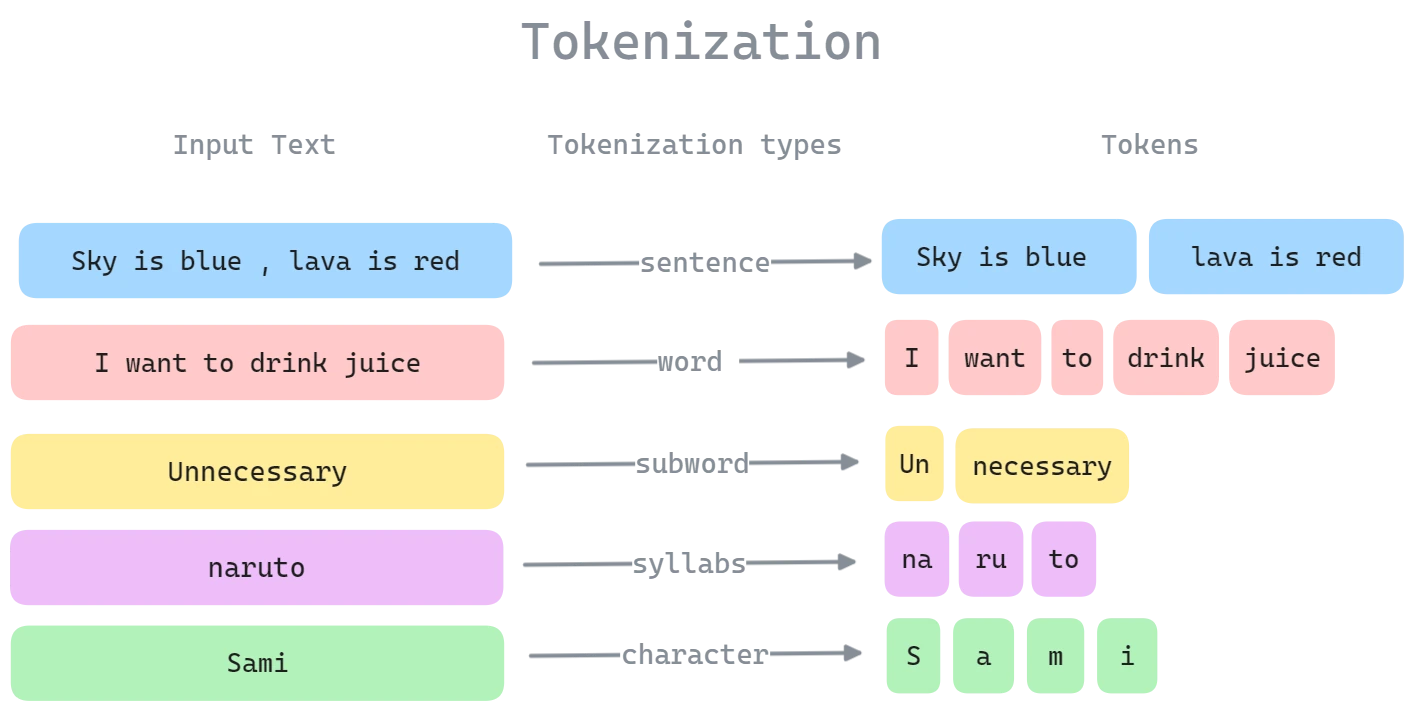Figure 1.0: Different tokenization strategies

The Tokenization Decision Matrix

The choice of tokenization strategy forces a fundamental trade-off:

• Word-level: Semantic clarity vs. vocabulary explosion and OOV failures
• Character-level: No OOV vs. sequence length explosion and inefficient learning
• Subword-level: Balance both vs. fragmentation, semantic blurring, and language bias

BPE (Byte-Pair Encoding): Learning the Vocabulary

BPE learns a vocabulary by discovering which character and subword pairs appear frequently together in training text. The algorithm is simple but powerful:

Process:

1. Initialize vocabulary with all characters in the text
2. Count how many times each adjacent pair of tokens appears
3. Merge the most frequent pair into a single token
4. Repeat until vocabulary reaches desired size

Why this works:

Frequent pairs are likely to represent meaningful units. By learning these merges from data, BPE discovers the tokenization that minimizes total sequence length while maintaining semantic information.

Example:

Initial: "h e l l o" (5 character tokens)
Iteration 1: "h e" appears 10 times → merge to "he"
Result: "he l l o"

Iteration 2: "l l" appears 8 times → merge to "ll"  
Result: "he ll o"

Iteration 3: "he l l o" → "ll o" appears 6 times → merge to "llo"
Result: "he llo"

Each merge decision is preserved in the vocabulary. At inference time, the learned merges are applied in order to tokenize new text.

Critical insight: BPE’s learned vocabulary is data-dependent. A vocabulary trained on medical text tokenizes differently than one trained on code. This means tokenization is tightly coupled to your training data distribution.

def learn_bpe(text, num_merges):
    # Initialize vocabulary with characters
    vocab = {c: text.count(c) for c in set(text)}
    pairs = get_stats(vocab)
    
    for i in range(num_merges):
        if not pairs:
            break
        best = max(pairs, key=pairs.get)
        vocab = merge_vocab(best, vocab)
        pairs = get_stats(vocab)
    
    return vocab

def get_stats(vocab):
    pairs = {}
    for word, freq in vocab.items():
        symbols = word.split()
        for i in range(len(symbols)-1):
            pair = (symbols[i], symbols[i+1])
            pairs[pair] = pairs.get(pair, 0) + freq
    return pairs

def merge_vocab(pair, vocab):
    new_vocab = {}
    bigram = ' '.join(pair)
    replacement = ''.join(pair)
    
    for word, freq in vocab.items():
        new_word = word.replace(bigram, replacement)
        new_vocab[new_word] = freq
    return new_vocab

Metrics for Evaluating Tokenization Quality

Unsupervised Metrics:

1. Compression Ratio: \(C = \frac{\text{total characters}}{\text{total tokens}}\) Measures information density per token. Higher is better. English typically achieves $C \approx 4-5$ with subword tokenization.

2. Vocabulary Coverage: \(\text{Coverage} = \frac{\text{unique tokens seen in training}}{V}\) Measures what fraction of the vocabulary is actually used. Coverage <80% suggests inefficient vocabulary allocation.

3. Out-of-Vocabulary Rate (OOV): \(\text{OOV rate} = \frac{\text{tokens not in vocabulary during inference}}{n}\) Should be <1% for well-designed tokenizers on in-domain text. High OOV indicates poor generalization.

4. Subword Fragment Rate: \(\text{Fragment rate} = \frac{\text{count of subword fragments (##tokens)}}{n}\) Lower is better. Fragment rate >40% indicates excessive morphological fragmentation.

5. Semantic Preservation (Normalized Pointwise Mutual Information): For semantically related words $w_1, w_2$ with tokenizations $T(w_1), T(w_2)$: \(\text{NPMI} = \frac{\text{PMI}(T(w_1), T(w_2))}{\text{max PMI}}\) Measures if related words share token patterns. Higher values indicate preserved semantic structure.

Supervised Metrics:

1. Downstream Task Performance: Train a language model on tokenized text and measure:
   • Perplexity: $\text{PPL} = \exp(-\frac{1}{n}\sum_{i=1}^n \log P(z_i))$
   • BLEU (for translation)
   • F1 (for sequence tagging)

Better downstream performance suggests tokenization preserves task-relevant information.

1. Task-Specific Generalization: Fine-tune on tokenized data; evaluate on:
   • Domain transfer accuracy (in-domain vs. out-of-domain)
   • Few-shot learning performance
   • Zero-shot transfer to unseen domains

Tokenization that generalizes well has minimal domain-dependence.

1. Arithmetic Benchmark (for numeric sensitivity): Evaluate on tasks like:
   • Simple arithmetic: “5 + 3 = ?”
   • Numerical comparison: “Which is larger: 3.14159 or 3.14160?”
   • Quantitative reasoning: “If x = 10, what is 2x + 5?”

Track accuracy as precision increases. Well-tokenized models maintain >90% accuracy on 4-digit arithmetic.

Special Tokens: Purpose and Impact

Beyond regular vocabulary tokens, models require special tokens for structural and handling purposes:

Types of Special Tokens:

1. ** (Padding Token)**
   • Purpose: Fill sequences to uniform length in batches
   • Why needed: Neural networks require fixed-size inputs. Different texts have different lengths. Padding makes all sequences the same length.
   • Example:

     Text: "hello world"
     Tokens: [101, 2054, 2088]
     Max length: 5
     Padded: [101, 2054, 2088, 0, 0]  (0 is <PAD> token ID)
     

   • Impact: Padding tokens consume attention computation but contribute no signal. Excessive padding reduces efficiency. Use attention masks to ignore padding.
2. ** (Unknown Token)**
   • Purpose: Represent words not in vocabulary
   • Why needed: Handles OOV problem. Without , the tokenizer has no representation for unknown words.
   • Trade-off: Using loses information (all unknown words map to same token). Better approach: use character-level fallback or BPE subword tokenization.
   • Impact: High frequency indicates poor vocabulary coverage. Models struggle to generalize to out-of-domain text.
3. ** / (Beginning/End of Sequence)**
   • Purpose: Mark sequence boundaries
   • Why needed: Tells the model where sequences start/end. Helps with generation tasks and bidirectional encoding.
   • Example (for generation):

     Input: <BOS> hello world <EOS>
     Model learns: "after <BOS>, predict 'hello'"
     "after 'world', predict <EOS>"
     

   • Impact: Essential for sequence generation. Models without boundary tokens struggle with knowing when to stop generating.
4. ** / (Classification / Separator)**
   • Purpose: Mark structure in sequences
   • Why needed: In BERT-style models, aggregates sequence representation for classification. separates multiple sequences.
   • Example (sentence pair classification): ```
   sentence A sentence B The model uses embedding for classification ``` - **Impact:** Allows single model to handle variable-length inputs and multi-sequence tasks.
5. ** (Masking Token)**
   • Purpose: Mark positions for masked language modeling
   • Why needed: During training, random tokens are replaced with to teach the model to predict masked words from context.
   • Example:

     Original: "The cat sat on the mat"
     Masked: "The [MASK] sat on the mat"
     Model predicts: "cat"
     

   • Impact: Enables self-supervised pre-training. Forces the model to learn bidirectional context.

Metrics for Special Token Usage:

• ** efficiency:** Measure average padding ratio = (total padding tokens) / (total tokens). Should be <10%. High ratio indicates inefficient batching.
• ** frequency:** Count (total tokens) / (total tokens). Should be <1%. >5% indicates vocabulary issues.
• **/ correctness:** Verify model learns to predict at sequence end. Plot attention to boundary tokens—well-trained models attend heavily to boundaries.
• ** representation quality:** For classification, measure if embedding alone achieves 90%+ accuracy on downstream tasks.

Practical Tips for Special Tokens:

• Use attention masks with tokens. Set attention weights to 0 for padding positions to prevent spurious attention patterns.
• Avoid mapping too many words to . If frequency >3%, expand vocabulary or use subword fallback.
• For multilingual models, use language-specific tokens if needed: , , etc. This helps the model track code-switching.
• and tokens are architecture-specific. Only use if your model is designed for them (e.g., BERT). Transformer-based models may not need them.
• During inference, always begin with and terminate on for generation tasks. Forgetting this causes infinite generation loops.
• Monitor which special tokens the model attends to. Excessive attention to indicates the model isn't learning meaningful patterns.

Edge Cases in Tokenization

1. Numbers and Mathematical Expressions

Numbers are fragmented across tokens:

"3.14159" → ["3", ".", "14", "159"]  (GPT-3 tokenizes π inefficiently)
"2+2=4" → ["2", "+", "2", "=", "4"]

This forces the model to learn numerical reasoning piecemeal. The model must maintain context across token fragments to understand that these are numbers, creating unnecessary cognitive load.

Impact on LLMs: Models struggle with arithmetic, quantitative reasoning, and scientific notation. They often “hallucinate” numbers because the fragmentation makes learning numerical patterns harder.

2. Code and Special Syntax

Programming languages tokenize inefficiently:

"if __name__ == '__main__':" fragments heavily
Indentation and whitespace become separate tokens

Impact on LLMs: Code generation is weaker than natural language because the tokenization doesn’t respect code structure. Related functions fragment across tokens.

3. Whitespace and Special Characters

Different tokenizers handle whitespace differently:

"hello world" might tokenize as:
GPT-3: ["hello", "world"]
BERT: ["hello", "world"]  (but respects different whitespace as separate tokens in some cases)

Some tokenizers preserve whitespace information; others strip it. This affects the model’s ability to understand formatting.

4. Language and Script Boundaries

Multilingual tokenizers face hard choices:

"café" (with composed accent) vs. "cafe" (with combining accent)
Different Unicode normalizations tokenize differently

Non-Latin scripts (Chinese, Arabic) are tokenized character-by-character or with special subword strategies because they don’t have clear word boundaries.

Impact on LLMs: Multilingual models are inherently imbalanced. English-heavy training data produces vocabularies that tokenize English efficiently but fragment non-Latin languages, forcing multilingual models to dedicate more parameters to low-resource languages.

Text Embedding

What is Text Embedding?

After tokenization, each token is just an integer. Neural networks cannot learn directly from these raw IDs—they need numerical representations that capture semantic meaning. Text embedding converts token IDs into dense vectors in a continuous vector space where semantically similar tokens are close together.

The embedding acts as a lookup table: given a token ID, retrieve its corresponding vector. This vector encodes what the model “knows” about that token.

One-Hot Encoding: The Baseline

Definition: Each token is represented as a vector of length $V$ (vocabulary size) with a 1 in the position corresponding to that token and 0s everywhere else.

\[\text{one\_hot}(w_i) = [0, \ldots, 1, \ldots, 0]\]

For vocabulary size 50,000: each token becomes a 50,000-dimensional vector with 99.998% zeros.

Why this is problematic:

• Sparsity: Massive vectors with mostly zeros waste memory and computation
• No semantic information: The vector encodes identity only, not meaning. “cat” and “dog” are orthogonal—equally far from each other as “cat” and “xyzzy”
• Scales poorly: Embedding dimension = vocabulary size. A 100,000-word vocabulary requires 100,000-dimensional vectors

Impact on LLMs: One-hot encoding is unused in modern LLMs because it provides no semantic structure. The model cannot leverage the fact that “cat” and “dog” are related animals.

Learned Dense Embeddings: The Standard

Definition: Each token maps to a learned vector of fixed size (typically 768-4096 dimensions). These vectors are learned during training.

\[\text{embed}(w_i) = E[w_i] \in \mathbb{R}^{d_{model}}\]

Where $E$ is an embedding matrix of shape $[V, d_{model}]$.

What the model learns: During training, the model adjusts these embedding vectors to make semantically related tokens have similar vector representations. This happens automatically through backpropagation—no explicit instruction needed.

Example: After training, vectors might satisfy: \(\text{embed}(\text{"king"}) - \text{embed}(\text{"man"}) + \text{embed}(\text{"woman"}) \approx \text{embed}(\text{"queen"})\)

Critical dependency on tokenization:

The quality of embeddings is constrained by tokenization. Consider two scenarios:

Scenario A: Good tokenization

Input: "The cat sat"
Tokens: ["The", "cat", "sat"]
Embeddings: 3 vectors to learn relationships between
Model: Learns "cat" and "sat" are both entities/actions

Scenario B: Bad tokenization (subword fragmentation)

Input: "The cat sat"
Tokens: ["The", "c", "##at", "s", "##at"]
Embeddings: 5 vectors, including meaningless subword pieces
Model: Must learn that "c" + "##at" = concept of "cat"
This wastes embedding capacity and learning signal

In scenario B, the model wastes capacity learning that certain subword combinations mean “cat” when that should have been a single token. This leaves less capacity for actually useful semantic patterns.

Metrics for Evaluating Embedding Quality

Unsupervised Metrics (Intrinsic Evaluation):

1. Semantic Similarity Correlation: Given a benchmark of word pairs with human-assigned similarity scores, compute: \(\rho = \text{Spearman correlation}(\text{cosine\_similarity}(e(w_1), e(w_2)), \text{human\_scores})\) Standard benchmarks: SimLex-999, RW, MTurk-771. Typical good embeddings achieve $\rho > 0.6$.

2. Word Analogy Accuracy: Test if embeddings satisfy: $e(\text{“king”}) - e(\text{“man”}) + e(\text{“woman”}) \approx e(\text{“queen”})$ \(\text{Accuracy} = \frac{\text{correct analogies}}{\text{total analogies}} \times 100\%\) Good embeddings achieve >70% accuracy on analogy tasks. This measures if semantic relationships are preserved.

3. Embedding Space Isotropy: \(\text{Isotropy} = \frac{1}{d} \sum_{i=1}^d \cos(\lambda_i, e_i)\) where $\lambda_i$ are eigenvectors of the embedding covariance matrix. More isotropic embeddings (closer to 1) distribute information uniformly; anisotropic embeddings waste dimensions.

4. Coverage of Subword Fragments: For subword tokens, measure if their embeddings form a coherent subspace: \(\text{Coherence} = \text{avg cosine\_similarity}(e(\text{##ing}), \text{prefix tokens})\) Low coherence indicates fragmented embeddings; high coherence suggests learned composition structure.

Supervised Metrics (Extrinsic Evaluation):

1. Downstream Task Performance: Use embeddings as input to downstream classifiers:
   • Text classification accuracy
   • Sentiment analysis F1
   • Named entity recognition (NER) precision/recall

Benchmark datasets: AG News, Movie Reviews, CoNLL-NER. Good embeddings achieve >85% accuracy on standard benchmarks.

1. Transfer Learning Efficiency: Train on task A, evaluate on task B: \(\text{Transfer ratio} = \frac{\text{accuracy with pretrained embeddings}}{\text{accuracy with random embeddings}}\) Ratio >1.5 indicates embeddings capture task-relevant features.

2. Compositional Generalization: For subword-tokenized models, test if composed embeddings work: \(\text{Composition error} = ||\text{compose}(e(z_1), e(z_2)) - e(\text{target})||_2\) Lower error indicates embeddings compose meaningfully.

3. Robustness to Out-of-Vocabulary Words: When encountering OOV words during inference:

   • Measure performance drop compared to in-vocabulary baseline
   • Track if composition strategy (sum/average/attention) recovers semantics

Well-designed embeddings degrade <5% when encountering OOV words.

Practical Tips for Text Embeddings:

• Choose embedding dimension based on vocabulary size: dimension ≈ log(vocabulary_size) × 50 is a reasonable heuristic. Too small causes information bottleneck; too large causes overfitting.
• Initialize embeddings with small random values around 0 (e.g., uniform(-0.1, 0.1)). Large initializations cause gradient issues.
• Use embedding regularization (L2 penalty) to prevent embeddings from growing unbounded during training.
• For OOV words, use character-level convolution or subword averaging, not a single <UNK> token. Single tokens lose information.
• Periodically evaluate embeddings on intrinsic benchmarks (analogy, similarity tasks) separate from downstream tasks.
• If downstream performance plateaus, the bottleneck may be embedding capacity, not model architecture. Try increasing embedding dimension.
• For multilingual models, consider separate embedding matrices per language or shared embeddings with language-specific projection layers.

Word2Vec Implementation:

class SkipGram(nn.Module):
    def __init__(self, vocab_size, embedding_dim):
        super(SkipGram, self).__init__()
        self.embeddings = nn.Embedding(vocab_size, embedding_dim)
        self.output = nn.Linear(embedding_dim, vocab_size)
        
    def forward(self, x):
        embed = self.embeddings(x)
        out = self.output(embed)
        return F.log_softmax(out, dim=1)

Positional Encoding

To capture word order in sequences, positional encoding adds position information to embeddings:

\(PE_{(pos,2i)} = \sin(pos/10000^{2i/d_{model}})\) \(PE_{(pos,2i+1)} = \cos(pos/10000^{2i/d_{model}})\)

Where:

• $pos$ is the position in the sequence
• $i$ is the dimension
• $d_{model}$ is the embedding dimension

def positional_encoding(max_seq_len, d_model):
    pe = torch.zeros(max_seq_len, d_model)
    position = torch.arange(0, max_seq_len, dtype=torch.float).unsqueeze(1)
    div_term = torch.exp(torch.arange(0, d_model, 2).float() * (-math.log(10000.0) / d_model))
    
    pe[:, 0::2] = torch.sin(position * div_term)
    pe[:, 1::2] = torch.cos(position * div_term)
    
    return pe

Attention Mechanism

Attention allows the model to focus on relevant parts of the input sequence. The scaled dot-product attention is defined as:

\[\text{Attention}(Q, K, V) = \text{softmax}\left(\frac{QK^T}{\sqrt{d_k}}\right)V\]

Where:

• $Q$ is the query matrix
• $K$ is the key matrix
• $V$ is the value matrix
• $d_k$ is the dimension of the keys

Attention enables language models to focus on crucial parts of a sentence, considering context. This allows them to grasp complex language, long-range connections, and word ambiguity.

Multi-Head Attention Implementation:

class MultiHeadAttention(nn.Module):
    def __init__(self, d_model, num_heads):
        super(MultiHeadAttention, self).__init__()
        self.num_heads = num_heads
        self.d_model = d_model
        
        assert d_model % num_heads == 0
        self.d_k = d_model // num_heads
        
        self.W_q = nn.Linear(d_model, d_model)
        self.W_k = nn.Linear(d_model, d_model)
        self.W_v = nn.Linear(d_model, d_model)
        self.W_o = nn.Linear(d_model, d_model)
        
    def scaled_dot_product_attention(self, Q, K, V, mask=None):
        attn_scores = torch.matmul(Q, K.transpose(-2, -1)) / math.sqrt(self.d_k)
        
        if mask is not None:
            attn_scores = attn_scores.masked_fill(mask == 0, -1e9)
            
        attn_probs = F.softmax(attn_scores, dim=-1)
        output = torch.matmul(attn_probs, V)
        return output
        
    def forward(self, Q, K, V, mask=None):
        batch_size = Q.size(0)
        
        # Linear projections
        Q = self.W_q(Q).view(batch_size, -1, self.num_heads, self.d_k).transpose(1, 2)
        K = self.W_k(K).view(batch_size, -1, self.num_heads, self.d_k).transpose(1, 2)
        V = self.W_v(V).view(batch_size, -1, self.num_heads, self.d_k).transpose(1, 2)
        
        # Apply attention on all the projected vectors in batch
        x = self.scaled_dot_product_attention(Q, K, V, mask)
        
        # Concatenate and apply final linear layer
        x = x.transpose(1, 2).contiguous().view(batch_size, -1, self.d_model)
        return self.W_o(x)

Text Preprocessing Operations

Let me explain each of these text processing concepts in simple terms:

1. Cleaning:

• Removing special characters: Getting rid of @#$%, punctuation marks, emojis, etc.

  text = text.replace('@#$%', '')  # Basic example
  

• Handling case sensitivity: Making all text either lowercase or uppercase so “Hello” and “hello” are treated the same

  text = text.lower()  # Convert to lowercase
  

• Removing stop words: Eliminating common words like “the”, “is”, “at” that don’t add much meaning

  from nltk.corpus import stopwords
  stop_words = set(stopwords.words('english'))
  text = [word for word in text if word not in stop_words]
  

2. Normalization:

• Lemmatization: Converting words to their dictionary base form

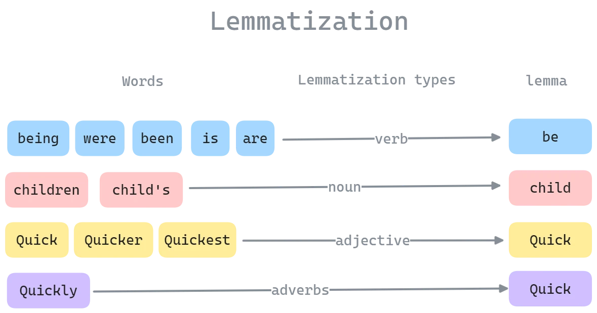Figure 2.0: Lemmatization process

  from nltk.stem import WordNetLemmatizer
  lemmatizer = WordNetLemmatizer()
  word = lemmatizer.lemmatize("running")  # Returns "run"

• Stemming: Cutting off word endings to get a common base (faster but rougher than lemmatization)

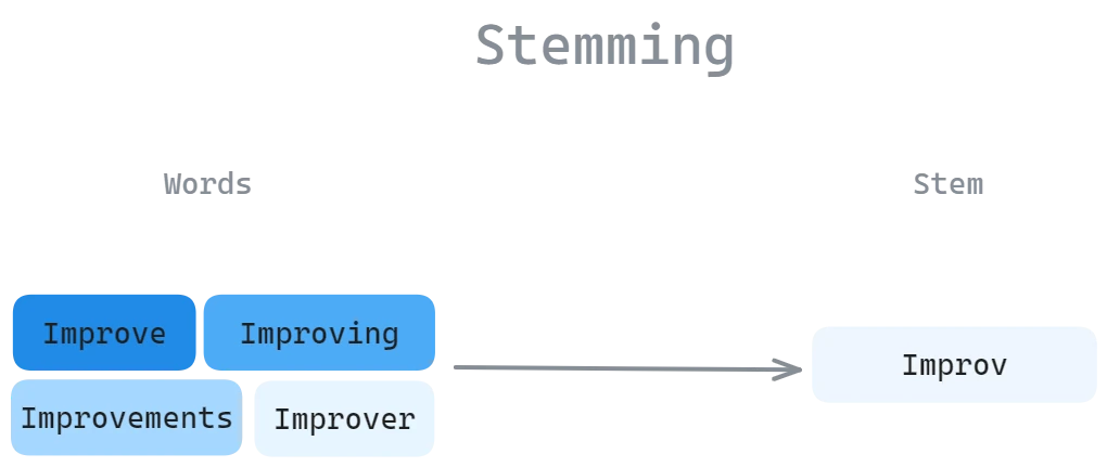Figure 3.0: Stemming process

  from nltk.stem import PorterStemmer
  stemmer = PorterStemmer()
  word = stemmer.stem("fishing")  # Returns "fish"

• Unicode normalization: Making sure similar characters are treated the same
  • “café” and “café” look same but might use different encodings

    import unicodedata
    text = unicodedata.normalize('NFKD', text)
    

These steps help prepare text data for analysis by making it more consistent and removing noise.

Advanced Text Operations

Text Augmentation

Text augmentation techniques help increase dataset size and improve model robustness:

1. Synonym Replacement: Replace words with their synonyms

2. Back Translation: Translate text to another language and back

3. Random Insertion/Deletion: Randomly insert or delete words while preserving meaning

def synonym_replacement(text, n=1):
    words = text.split()
    new_words = words.copy()
    random_word_list = list(set([word for word in words]))
    num_replaced = 0
    
    for random_word in random_word_list:
        synonyms = []
        for syn in wordnet.synsets(random_word):
            for l in syn.lemmas():
                synonyms.append(l.name())
                
        if len(synonyms) >= 1:
            synonym = random.choice(list(set(synonyms)))
            new_words = [synonym if word == random_word else word for word in new_words]
            num_replaced += 1
        
        if num_replaced >= n:
            break
            
    return ' '.join(new_words)

Sequence Padding

To handle variable-length sequences in batches, padding is used to make all sequences the same length:

def pad_sequences(sequences, max_len=None, padding='post'):
    if max_len is None:
        max_len = max(len(seq) for seq in sequences)
        
    padded_sequences = []
    for seq in sequences:
        if len(seq) < max_len:
            if padding == 'post':
                padded_seq = seq + [0] * (max_len - len(seq))
            else:  # pre-padding
                padded_seq = [0] * (max_len - len(seq)) + seq
        else:
            padded_seq = seq[:max_len]
        padded_sequences.append(padded_seq)
        
    return torch.tensor(padded_sequences)

Why Text Operations Matter

Text operations determine model capability. Poor implementation cascades through the entire architecture.

• Information Efficiency: Tokenization determines how much meaning fits in the context window. Efficient tokenization (high compression ratio) lets models see more content; inefficient tokenization wastes tokens on fragments.
• Semantic Preservation: Embeddings encode whether the model understands relationships between words. Well-designed embeddings capture that “king - man + woman ≈ queen”; poor embeddings treat all words as independent.
• Structural Integrity: Lemmatization and stemming reduce noise by recognizing that “being, were, been, is, are” all represent the same verb “be.” This forces the model to learn patterns on unified concepts, not scattered variants.
• Downstream Performance: Models cannot exceed the quality of their text operations. A well-tokenized, well-embedded input enables strong performance; fragmented, poorly-embedded input limits all downstream tasks regardless of architecture quality.

---

Reference:

• Attention Is All You Need
• Word2Vec
• BERT