Model entanglement
Explaining what can impact changes in a model and why technical debt is detrimental.
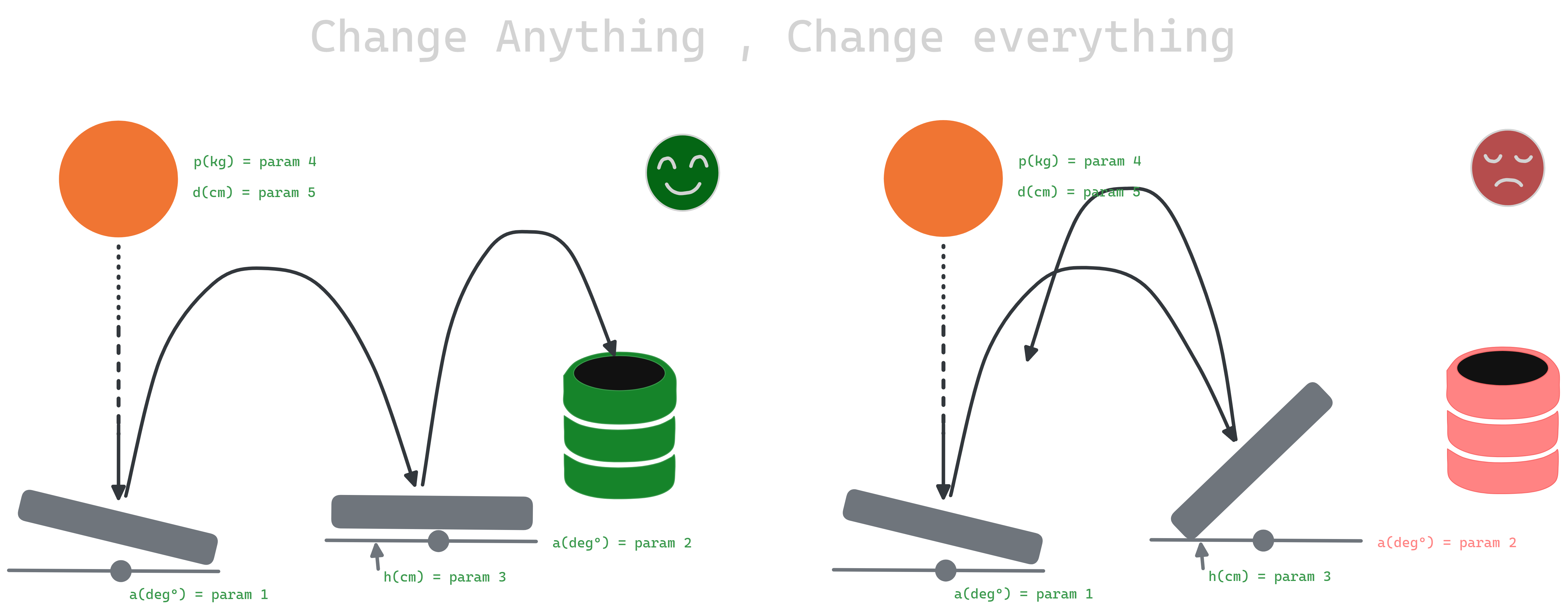 Figure 0.1: Model entanglement and CACE principle illustration
Entanglement in Machine Learning Models and the “CACE Principle”
In machine learning, entanglement refers to the complex interdependencies between features, where modifying one feature can affect the behavior of others. This phenomenon is captured by the “CACE Principle” (Changing Anything Changes Everything) also called “cake” principle 🎂, which highlights how altering any feature can influence the model’s overall predictions.
Machine learning models use a set of features \(x_1, x_2, \dots, x_n\), and the relationships between them are often non-linear. Any change, such as shifts in input distribution, adding new features, or removing existing ones, can disrupt the model’s learned dynamics.
Types of Feature Changes:
Input Distribution Change: A shift in how feature values are distributed can alter the model’s weighting of other features.
Adding a New Feature \(x_{n+1}\): Introducing new data alters the balance of the model, potentially impacting existing features.
Removing a Feature \(x_j\): Excluding a feature forces the model to redistribute its reliance on remaining features, often unpredictably.
Mitigation Strategies:
- Feature Interaction Monitoring: Track how features affect one another to detect potential issues early.
- Regularization: Use techniques like L1/L2 regularization to control feature influence.
- Retraining: Regularly retrain the model after any changes to ensure stability.
By recognizing and addressing feature entanglement, models can maintain accuracy and predictability even as features evolve.
Workshop
1. Model Development
IN[1] :
1
2
3
4
5
6
7
8
9
10
11
12
13
14
15
16
17
18
19
20
21
22
23
24
25
26
27
28
29
import numpy as np
import pandas as pd
from sklearn.tree import DecisionTreeClassifier
from sklearn.model_selection import train_test_split
from sklearn.metrics import accuracy_score

# Generate synthetic dataset
np.random.seed(42)
n_samples = 1000

# Features: x1, x2, x3
x1 = np.random.normal(loc=0, scale=1, size=n_samples)  # Normally distributed feature
x2 = np.random.uniform(0, 1, size=n_samples)           # Uniformly distributed feature
x3 = np.random.poisson(lam=3, size=n_samples)          # Poisson distributed feature

# Target variable (binary classification)
y = (x1 + x2 + x3 > 3).astype(int)

# Create a DataFrame
df = pd.DataFrame({'x1': x1, 'x2': x2, 'x3': x3, 'y': y})

# Train-test split
X = df[['x1', 'x2', 'x3']]
y = df['y']
X_train, X_test, y_train, y_test = train_test_split(X, y, test_size=0.3, random_state=42)

# Train initial model
model = DecisionTreeClassifier(random_state=42)
model.fit(X_train, y_train)
OUT[1] :
 Figure 1.0: Decision tree classifier visualization
Initial Loss Function (Cross-Entropy Loss)
The cross-entropy loss for a classification problem can be represented as:
\[\mathcal{L} = -\frac{1}{N} \sum_{i=1}^{N} \left[ y_i \log(\hat{y}_i) + (1 - y_i) \log(1 - \hat{y}_i) \right]\]where:
- \(N\) is the total number of samples,
- \(y_i\) is the true label of sample \(i\),
- \(\hat{y}_i\) is the predicted probability of the positive class for sample \(i\).
2. Model Evaluation
IN[2] :
1
2
y_pred = model.predict(X_test)
print(f"Initial Accuracy: {accuracy_score(y_test, y_pred):.4f}")
OUT[2] :
1
Initial Accuracy: 0.9433
Loss After Feature Modification
Change in Input Distribution: Let \(x_1' = x_1 + \Delta x_1\) represent the shifted feature. The new model predictions will depend on this change, and the new loss becomes:
\[\mathcal{L'} = -\frac{1}{N} \sum_{i=1}^{N} \left[ y_i \log(\hat{y}'_i) + (1 - y_i) \log(1 - \hat{y}'_i) \right]\]where \(\hat{y}'_i\) represents the updated predictions based on the shifted feature \(x_1'\).
Adding a New Feature: If we add a new feature \(x_{n+1}\), the model updates its predictions to account for this new feature. The updated loss can be written as:
\[\mathcal{L''} = -\frac{1}{N} \sum_{i=1}^{N} \left[ y_i \log(\hat{y}''_i) + (1 - y_i) \log(1 - \hat{y}''_i) \right]\]where \(\hat{y}''_i\) is the prediction made by the model after incorporating the new feature \(x_{n+1}\).
Removing a Feature: If we remove feature \(x_j\), the model must make predictions based on the remaining features. The new loss is:
\[\mathcal{L^{(j)}} = -\frac{1}{N} \sum_{i=1}^{N} \left[ y_i \log(\hat{y}^{(j)}_i) + (1 - y_i) \log(1 - \hat{y}^{(j)}_i) \right]\]where \(\hat{y}^{(j)}_i\) are the predictions made without feature \(x_j\).
3. Change 1: Shift in input distribution of x1
IN[3] :
1
2
3
4
5
X_test_shifted = X_test.copy()
X_test_shifted['x1'] = X_test_shifted['x1'] + 1  # Shift the distribution of x1

y_pred_shifted = model.predict(X_test_shifted)
print(f"Accuracy after shifting x1: {accuracy_score(y_test, y_pred_shifted):.4f}")
OUT[3] :
1
Accuracy after shifting x1: 0.7833
4. Change 2: Add a new feature (x4)
IN[4] :
1
2
3
4
5
6
7
8
X_train['x4'] = np.random.normal(loc=0, scale=1, size=len(X_train))  # New feature x4
X_test['x4'] = np.random.normal(loc=0, scale=1, size=len(X_test))

model_with_new_feature = DecisionTreeClassifier(random_state=42)
model_with_new_feature.fit(X_train, y_train)

y_pred_new_feature = model_with_new_feature.predict(X_test)
print(f"Accuracy after adding new feature x4: {accuracy_score(y_test, y_pred_new_feature):.4f}")
OUT[4] :
1
Accuracy after adding new feature x4: 0.9433
5. Change 3: Remove a feature (x2)
IN[5] :
1
2
3
4
5
6
7
8
9
10
X_train_reduced = X_train.drop(columns=['x2'])
X_test_reduced = X_test.drop(columns=['x2'])

model_with_removed_feature = DecisionTreeClassifier(random_state=42)
model_with_removed_feature.fit(X_train_reduced, y_train)


y_pred_removed_feature = model_with_removed_feature.predict(X_test_reduced)
print(f"Accuracy after removing feature x2: {accuracy_score(y_test, y_pred_removed_feature):.4f}")
OUT[5] :
1
Accuracy after removing feature x2: 0.9200
Loss Difference:
The difference between the original loss \(\mathcal{L}\) and the loss after the feature modification can be expressed as:
\[\Delta \mathcal{L} = \mathcal{L'} - \mathcal{L}\]For each change (shift, addition, or removal), this loss difference quantifies the impact of the feature modification:
- After shifting \(x_1\): \(\Delta \mathcal{L}_1 = \mathcal{L'} - \mathcal{L}\)
- After adding \(x_{n+1}\): \(\Delta \mathcal{L}_2 = \mathcal{L''} - \mathcal{L}\)
- After removing \(x_j\): \(\Delta \mathcal{L}_3 = \mathcal{L^{(j)}} - \mathcal{L}\)
By analyzing \(\Delta \mathcal{L}\), we can observe how modifying features alters the model’s performance in terms of loss.
Reference :
- D. Sculley et al. « Hidden Technical Debt in Machine Learning Systems ». In : Advances in Neural Information Processing Systems (2015), p. 2503-2511.