Data drift overview
Writing on data drift and its various types
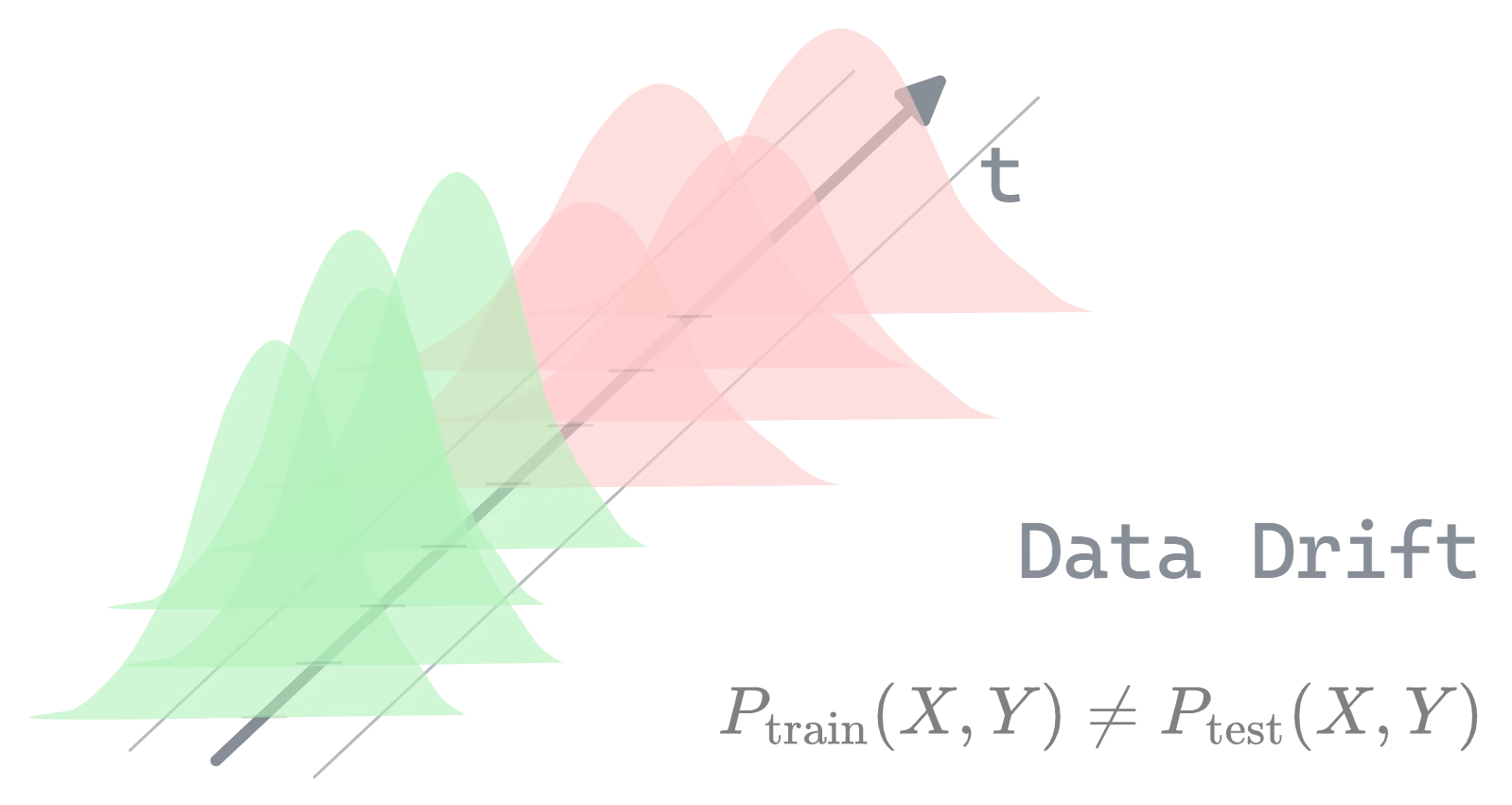 Figure 0.1: Data drift overview
What’s Data Drift ?
Data drift refers to the change in the statistical properties of input data over time, impacting the reliability of machine learning models. Unlike concept drift, which requires monitoring prediction performance through metrics like accuracy or precision, data drift can be detected by monitoring the stability of input features using statistical metrics.
History
The concept of data drift was recognized as machine learning and statistical models began to be applied in real-world settings, where data used to train models often changed over time.
While it’s difficult to pinpoint an exact date, data drift became a critical concept as models moved from static environments to dynamic, evolving data ecosystems, particularly with the rise of automated decision systems in industries like finance, healthcare, and technology in the late 1990s and early 2000s.
Stability-metric-for-data-drift
To ensure models remain accurate in production, stability metrics , they are used to detect changes in input data distributions, focusing on identifying covariate drift.
here’s how we can use stability metrics
- Detect changes in prior probability using metrics such as the Population Stability Index (PSI) and Divergence Index.
- Identify covariate shifts using tools like the Covariate Stability Index (CSI) and Novelty Index.
These metrics rely on both the input and output data in the production environment.
Types of Data Drift in Machine Learning
Notation :
- \(P_{\text{train}}\): Distribution of the training data
- \(P_{\text{test}}\): Distribution of the test or production data
- \(X\): Input variables (features)
- \(Y\): Target variable (to be predicted)
- \(C\): the counfounders or covariate
Mathematical Formulation :
\[P_{\text{train}}(X, Y) \neq P_{\text{test}}(X, Y)\]There’s 3 main subcategories (covariate shift , Prior probability shift & Sample Selection Bias:)
a) Covariate Shift:
Covariate shift occurs when the distribution of the input features (i.e., the characteristics or attributes) changes between the training and test data, but the way the features relate to the target (the thing you’re trying to predict) remains the same.
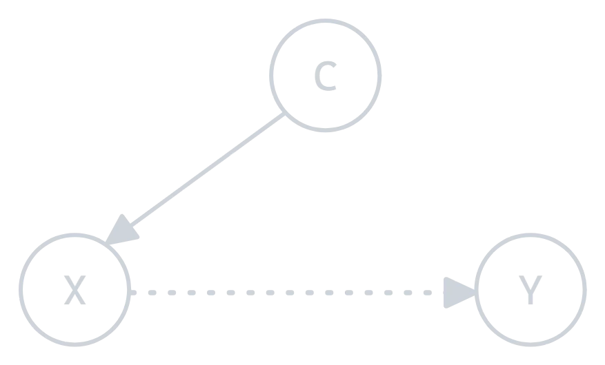 Figure 1.0: Covariate shift illustration
SubSubcategories:
1. Covariate Observation Shift (COS) Occurs when the conditional distribution of covariates given the labels shifts between training and testing:
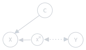 Figure 1.1: Covariate observation shift
- Example: A model trained on animal images in a controlled environment tested on outdoor images with different lighting conditions.
2. Covariate Hidden Shift (CHS) Involves the presence of a hidden variable \(X_H\) that alters the covariates. The conditional distribution of hidden covariates given the observed covariates changes:
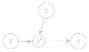 Figure 1.2: Covariate hidden shift
- Example: A sales prediction model trained without considering economic changes as a hidden variable.
3. Distorted Covariate Shift (DCS) Occurs when observed covariates are noisy or distorted compared to the true covariates:
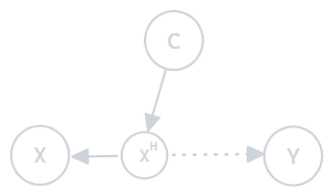 Figure 1.3: Distorted covariate shift
- Example: Faulty sensors in a manufacturing process providing inaccurate data to a predictive model.
b) Prior Probability Shift:
Prior probability shift happens when the overall proportion of the different classes or categories in the target variable changes between training and test data, but the relationship between the features and the target stays consistent.
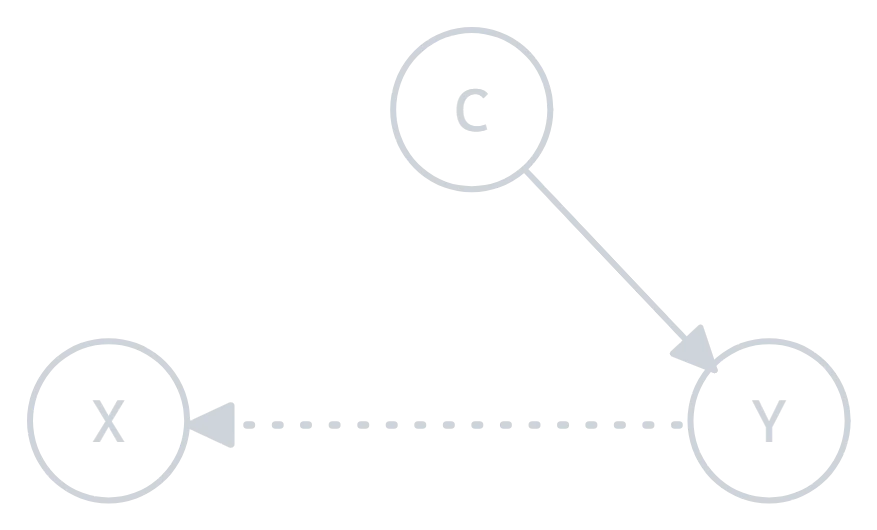 Figure 2.0: Prior probability shift illustration
1. Prior Probability Observation Shift (PPOS) Occurs when the prior probability distribution changes, and there is also an unobserved (hidden) factor \(X_H\) that affects the covariates. The relationship between the hidden covariate and the label changes:
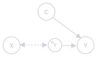 Figure 2.1: Prior probability observation shift
- Example: In a customer segmentation task, an unobserved variable like customer behavior changes over time, affecting the relationships between segments and their features.
2. Prior Probability Hidden Shift (PPHS) This type of shift occurs when a hidden variable \(X_H\) influences both the covariates and the labels, and its conditional distribution shifts between the training and test datasets:
Figure 2.2: Prior probability hidden shift
- Example: A medical model trained on data where \(X_H\) (e.g., certain health conditions) influences both the test results and the patient outcomes, but changes in how those conditions manifest over time cause a shift.
3. Distorted Prior Probability Shift (DPPS) Occurs when the prior probability distribution shifts and the covariates are distorted. The observed covariates do not match the true covariates:
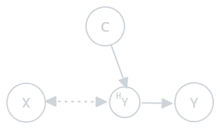 Figure 2.3: Distorted prior probability shift
- Example: A model trained with clean data might perform poorly when tested on noisy data, combined with a shift in label distributions. For instance, sensor errors distort the data, and class distributions also change.
c) Sample Selection Bias:
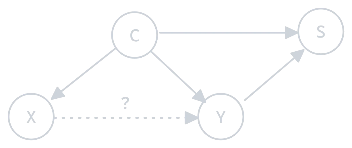 Figure 3.0: Sample selection bias illustration
Sample selection bias occurs when the training data is not representative of the real-world population, leading to incorrect conclusions because the data comes from a skewed subset.
- Target Population vs. Sampling Population:
- Target Population: This is the group you’re really interested in for your study.
- Sampling Population: This is the group from which your sample is actually drawn. Ideally, this group would match the target population. However, due to practical constraints or selection
- Selection Mechanism:
The selection mechanism refers to the factors that determine whether someone is included in your sample. It could involve different reasons, such as:- Refusal: People might refuse to participate in the study.
- Dropout: Some participants might leave the study before it’s completed.
- Death: In longitudinal studies, individuals might die before the study is complete, leading to their exclusion.
All of these factors cause the sampling population to be systematically different from the target population, introducing bias.
The Problem with Selection Bias:
The goal of most studies is to make conclusions about the target population. However, when there’s selection bias, the results of your analysis may only apply to the sampling population.- Stratum-Specific vs. Marginal Parameters:
The text uses a model to describe how outcomes differ between the sampling and target populations:- Stratum-specific parameters are estimates that apply only to those selected into the sample (S = 1). These reflect the relationships in the sampling population.
- Marginal parameters are estimates that average over both selected (S = 1) and non-selected individuals (S = 0), reflecting the relationships in the target population. Selection bias occurs when you want to estimate the marginal parameters (target population), but your data only provides stratum-specific parameters (sampling population).
Reference :
- Joaquin Quiñonero-Candela et al., éd. Dataset Shift in Machine Learning. Cambridge, MA, USA : MIT Press, 2009. isbn : 9780262170055.
- Haneuse, S., Schildcrout, J., Crane, P., Sonnen, J., Breitner, J., & Larson, E. (2009). Adjustment for Selection Bias in Observational Studies with Application to the Analysis of Autopsy Data. Neuroepidemiology, 32, 229-39. https://doi.org/10.1159/000197389