Convolutional neural networks
Describing Convolutional neural networks

Overview
Convolutional Neural Networks (ConvNets or CNNs) are a type of neural network where the primary operation is the convolution of data matrices. Technically, they use cross-correlation instead of convolution. Cross-correlation is similar to convolution, but without flipping the kernel. The kernel, a smaller matrix that moves over the input, performs the convolution operation to extract features.
How Convolution Works in CNNs:
The kernel overlaps with sections of the input matrix, and the dot product of each overlap is computed and summed. This process generates a feature map (such as a sharpened image). Convolution extracts significant features from the input, such as edges.
Why Use Convolutional Networks?
Sparse Interactions: ConvNets, using small kernels (of size $k$), require fewer computations than traditional neural networks. They reduce calculations from $m \times n$ to $k \times n$, where $m$ and $n$ represent the input and output sizes.
Parameter Sharing: In CNNs, the same set of parameters (the kernel) is applied to different parts of the input, promoting efficiency. In contrast, traditional neural networks use unique weights for different parts of the input, which are only applied once.
Equivariance: This means that if the input shifts, the output shifts in the same way. For example, if brightness is applied to a pixel and then the pixel is moved, applying the convolution again would reflect the brightness at the new location.
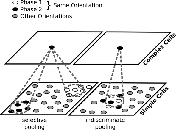
The Feature Extraction Mechanism in convolutional neural networks emulates the hierarchical processing of visual information in the human visual cortex, extracting increasingly complex features from the input data.
Before proceeding to implement ConvNets in PyTorch, there’s one more essential concept to cover.
CNN Operations
Convolution Operation
Origin
In mathematics (in particular, functional analysis), convolution is a mathematical operation on two functions (f

The convolution of two functions \(f\) and \(g\), written as \(f * g\), is defined as the integral of the product of \(f\) and a time-shifted, reflected version of \(g\):
\[(f * g)(t) = \int_{-\infty}^{\infty} f(\tau)g(t-\tau) \, d\tau\]An equivalent form is:
\[(f * g)(t) = \int_{-\infty}^{\infty} f(t-\tau)g(\tau) \, d\tau\]This describes how \(f\) is weighted by a shifted and flipped version of \(g\), and as \(t\) varies, the relative position of the two functions shifts.
Cross-correlation : The cross-correlation between two functions \(f(t)\) and \(g(t)\), denoted as \((f \star g)(t)\), is defined as:
\[(f \star g)(t) = \int_{-\infty}^{\infty} f(\tau) g(t + \tau) \, d\tau\]Autocorrelation : The autocorrelation of a function \(f(t)\), denoted as \(R_f(t)\), is a special case of cross-correlation where a function is correlated with itself:
\[R_f(t) = \int_{-\infty}^{\infty} f(\tau) f(t + \tau) \, d\tau\]Differences

Convolution: In convolution, one function is flipped (reflected) before being shifted and multiplied by the other. The formula involves \(g(t - \tau)\), which causes this reflection. It’s widely used in systems analysis (signal processing, linear systems) and has an inherent interpretation related to the response of systems.
Cross-correlation: Cross-correlation measures the similarity between two signals as one is shifted over the other without flipping. It helps to find patterns or matching features between signals and is often used in pattern recognition, feature matching, and alignment tasks.
Autocorrelation: Autocorrelation is a self-comparison of a signal with a shifted version of itself. It measures how similar a signal is to itself over different time lags. It’s used to detect repeating patterns, periodic signals, or noise within the signal.
The discrete convolution of two functions \(f\) and \(g\), for integers \(n\), is defined as:
\[(f * g)[n] = \sum_{m=-\infty}^{\infty} f[m]g[n - m]\]Or equivalently, by commutativity:
\[(f * g)[n] = \sum_{m=-\infty}^{\infty} f[n - m]g[m]\]For finite sequences (e.g., when \(g\) has finite support in \(\{-M, -M+1, \dots, M-1, M\}\)), the convolution becomes a finite sum:
\[(f * g)[n] = \sum_{m=-M}^{M} f[n - m]g[m]\]This describes how convolution can be extended to finitely supported sequences and relates to the Cauchy product of polynomials.
Convolution Layer
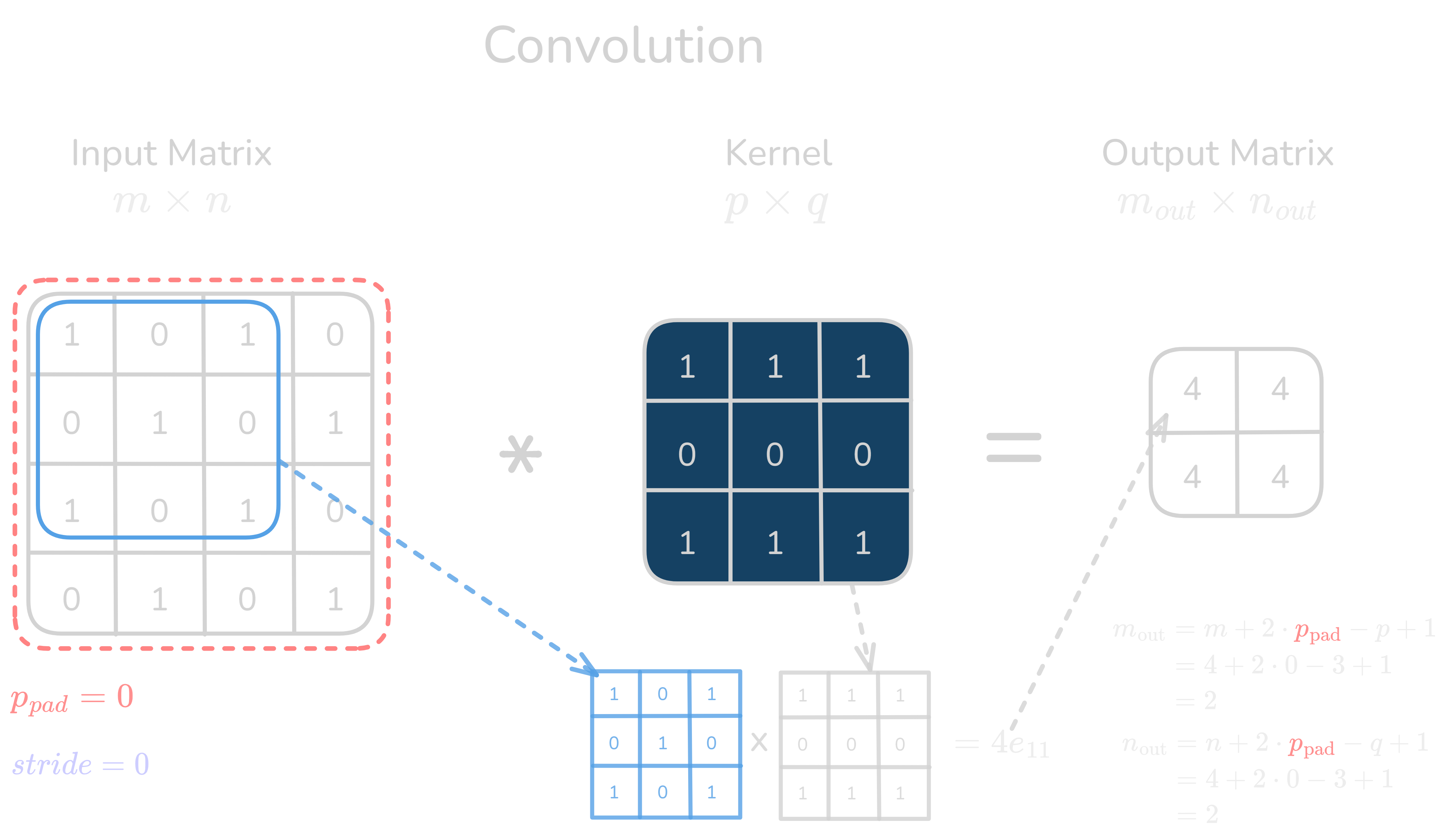 Figure 1.0: Convolution layer operation
- Output dimensions for convolution:
For a 2D convolution, the output matrix dimensions \(m_{\text{out}} \times n_{\text{out}}\) are determined by the following formulas:
\(m_{\text{out}} = \left\lfloor \frac{m + 2p_{\text{pad}} - p}{\text{stride}} \right\rfloor + 1\) \(n_{\text{out}} = \left\lfloor \frac{n + 2p_{\text{pad}} - q}{\text{stride}} \right\rfloor + 1\)
Where:
- \(m \times n\) are the dimensions of the input matrix.
- \(p \times q\) are the dimensions of the kernel.
- \(p_{\text{pad}}\) is the padding (the number of zeros added around the input matrix).
strideis the step size for moving the kernel across the input matrix.
- Convolution operation (element-wise):
For each position of the kernel on the input matrix, the value at a given position in the output matrix is computed as:
\[\text{Output}(i, j) = \sum_{\text{each element in the kernel}} \left( \text{Input}(i+k, j+l) \times \text{Kernel}(k, l) \right)\]
Example with Matrix Convolution (including padding and stride):
Let’s use an example where:
- Input matrix \(I\) is \(4 \times 4\).
- Kernel \(K\) is \(3 \times 3\).
- Padding \(p_{\text{pad}} = 1\).
- Stride \(\text{stride} = 2\).
Step 1: Input matrix and kernel
Input matrix \(I\): \(\begin{pmatrix} 1 & 0 & 1 & 0 \\ 0 & 1 & 0 & 1 \\ 1 & 0 & 1 & 0 \\ 0 & 1 & 0 & 1 \\ \end{pmatrix}\)
Kernel \(K\): \(\begin{pmatrix} 1 & 1 & 1 \\ 0 & 0 & 0 \\ 1 & 1 & 1 \\ \end{pmatrix}\)
Step 2: Apply padding
With padding \(p_{\text{pad}} = 1\), we add a 1-pixel border of zeros around the input matrix:
\[\begin{pmatrix} 0 & 0 & 0 & 0 & 0 & 0 \\ 0 & 1 & 0 & 1 & 0 & 0 \\ 0 & 0 & 1 & 0 & 1 & 0 \\ 0 & 1 & 0 & 1 & 0 & 0 \\ 0 & 0 & 1 & 0 & 1 & 0 \\ 0 & 0 & 0 & 0 & 0 & 0 \\ \end{pmatrix}\]Step 3: Perform convolution with stride
Since the stride is \(\text{stride} = 2\), the kernel moves 2 steps at a time across the padded input matrix.
Convolution at each position:
Position (0,0): \(\begin{pmatrix} 0 & 0 & 0 \\ 0 & 1 & 0 \\ 0 & 0 & 1 \\ \end{pmatrix} \cdot \begin{pmatrix} 1 & 1 & 1 \\ 0 & 0 & 0 \\ 1 & 1 & 1 \\ \end{pmatrix} = (0+0+0+0+0+0+0+0+1) = 1\)
Position (0,2): \(\begin{pmatrix} 0 & 0 & 0 \\ 0 & 1 & 0 \\ 1 & 0 & 1 \\ \end{pmatrix} \cdot \begin{pmatrix} 1 & 1 & 1 \\ 0 & 0 & 0 \\ 1 & 1 & 1 \\ \end{pmatrix} = (0+0+0+0+1+0+1+0+1) = 3\)
Position (2,0): \(\begin{pmatrix} 0 & 1 & 0 \\ 0 & 0 & 1 \\ 0 & 1 & 0 \\ \end{pmatrix} \cdot \begin{pmatrix} 1 & 1 & 1 \\ 0 & 0 & 0 \\ 1 & 1 & 1 \\ \end{pmatrix} = (0+1+0+0+0+0+0+1+0) = 2\)
Position (2,2): \(\begin{pmatrix} 1 & 0 & 1 \\ 0 & 1 & 0 \\ 1 & 0 & 1 \\ \end{pmatrix} \cdot \begin{pmatrix} 1 & 1 & 1 \\ 0 & 0 & 0 \\ 1 & 1 & 1 \\ \end{pmatrix} = (1+0+1+0+1+0+1+0+1) = 5\)
Step 4: Output matrix
\[\begin{pmatrix} 1 & 3 \\ 2 & 5 \\ \end{pmatrix}\]Thus, the output matrix after applying convolution with padding and stride is \(2 \times 2\). Here’s a PyTorch implementation of 2D convolution using the provided example, which includes padding and stride.
1
2
3
4
5
6
7
8
9
10
11
12
13
14
15
16
17
18
19
20
21
22
import torch.nn.functional as F

# Define the input matrix (4x4)
input_matrix = torch.tensor([[1, 0, 1, 0],
                             [0, 1, 0, 1],
                             [1, 0, 1, 0],
                             [0, 1, 0, 1]], dtype=torch.float32)

# Reshape to match PyTorch's expected input shape: (batch_size, channels, height, width)
input_matrix = input_matrix.unsqueeze(0).unsqueeze(0)  # Shape: (1, 1, 4, 4)

# Define the kernel (3x3)
kernel = torch.tensor([[1, 1, 1],
                       [0, 0, 0],
                       [1, 1, 1]], dtype=torch.float32)

# Reshape to match PyTorch's expected kernel shape: (out_channels, in_channels, height, width)
kernel = kernel.unsqueeze(0).unsqueeze(0)  # Shape: (1, 1, 3, 3)

# Apply 2D convolution using F.conv2d
# We use stride=2 and padding=1 as per the example
output = F.conv2d(input_matrix, kernel, stride=2, padding=1)
Pooling layer
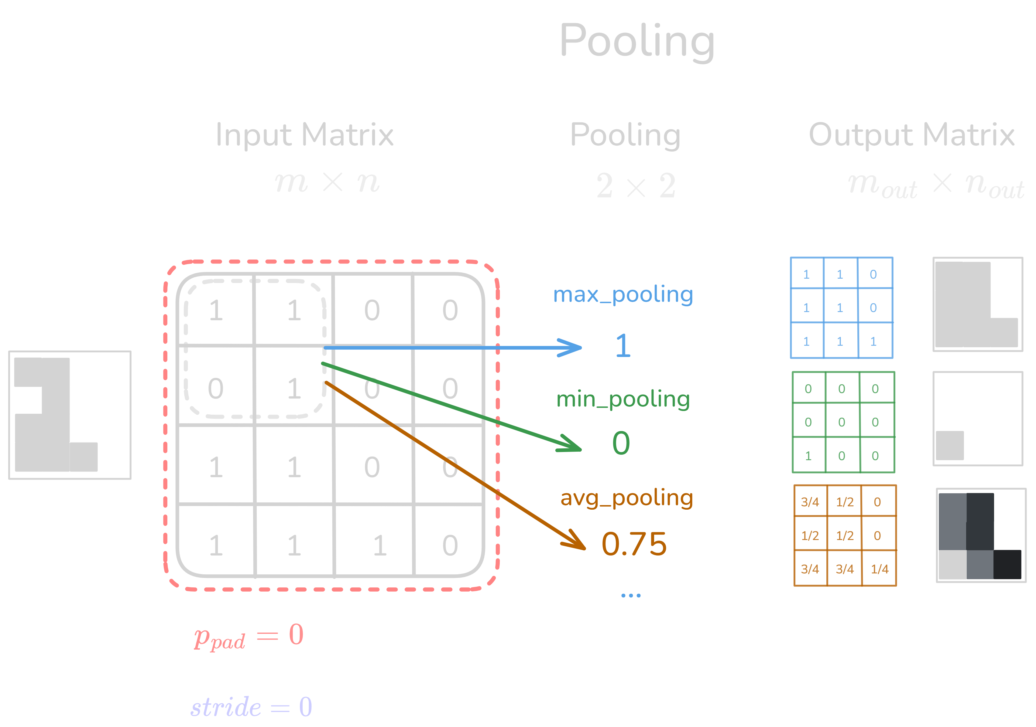 Figure 2.0: Pooling layer operation
Definition: Pooling is a down-sampling operation used in Convolutional Neural Networks (CNNs) to reduce the spatial dimensions of input feature maps (e.g., height and width), helping to retain key features while lowering computational costs. Pooling enhances model efficiency, aids in reducing overfitting, and promotes translation invariance by making the network less sensitive to small shifts in the input.
Pooling is generally performed over a window (or filter) of size \(k \times k\) across the input tensor. Given an input feature map \(S\) of size \(H \times W\) (height × width), pooling with filter size \(k \times k\), stride \(s\), and padding \(p\) can be described by the following general function:
\(f_{X,Y}(S) = \text{pool}\left( S_{X+s \cdot a : X+s \cdot (a+k), Y+s \cdot b : Y+s \cdot (b+k)} \right)\) where:
- \(f_{X,Y}(S)\) is the output of pooling at position \((X, Y)\).
- \(S_{X,Y}\) is the input value at the position \((X, Y)\).
- \(k\) is the size of the pooling filter (e.g., \(k = 2\) for a \(2 \times 2\) filter).
- \(s\) is the stride, which determines how much the filter moves along the input.
- \(p\) is the padding, which adds zeros around the input if necessary.
- \(a, b\) are the dimensions inside the pooling window.
- \(\text{pool}()\) is the pooling function applied to the region, depending on the type of pooling.
Pooling Subcategories, Features, and Formulas
- Max Pooling: Selects the maximum value from each pooling region. \(f_{X,Y}(S) = \max_{a,b} \left( S_{X + s \cdot a, Y + s \cdot b} \right)\) where \(a, b \in \{0, \dots, k-1\}\).
- Use Case: Useful for capturing the strongest activation in each region, leading to robust feature extraction.
- Average Pooling: Averages all the values within the pooling region. \(f_{X,Y}(S) = \frac{1}{k^2} \sum_{a=0}^{k-1} \sum_{b=0}^{k-1} S_{X + s \cdot a, Y + s \cdot b}\)
- Use Case: Historically used for smoothing, it is useful when all features in a region are of interest, not just the maximum.
- L2-Norm Pooling: Computes the L2 norm (Euclidean norm) of the values in the pooling region. \(f_{X,Y}(S) = \sqrt{\sum_{a=0}^{k-1} \sum_{b=0}^{k-1} \left( S_{X + s \cdot a, Y + s \cdot b} \right)^2}\)
- Use Case: Rarely used, but can be effective in applications requiring a magnitude-based summary of features in a region.
- Global Pooling (Global Max or Global Average Pooling):Applies pooling over the entire spatial dimensions (height and width) of the input, reducing the feature map to a single value per channel. \(f(S) = \frac{1}{H \times W} \sum_{X=0}^{H-1} \sum_{Y=0}^{W-1} S_{X,Y}\)
1
2
3
4
5
6
7
8
9
10
11
12
13
14
15
16
17
# Example input tensor (batch size: 1, channels: 1, height: 4, width: 4)
input_tensor = torch.tensor([[[[1.0, 2.0, 3.0, 0.0],
                               [4.0, 5.0, 6.0, 1.0],
                               [3.0, 4.0, 7.0, 2.0],
                               [1.0, 2.0, 1.0, 0.0]]]])

# Max Pooling (2x2 filter, stride 2, padding 0)
max_pooling = nn.MaxPool2d(kernel_size=2, stride=2, padding=0)
output_max = max_pooling(input_tensor)

# Average Pooling (2x2 filter, stride 2, padding 0)
avg_pooling = nn.AvgPool2d(kernel_size=2, stride=2, padding=0)
output_avg = avg_pooling(input_tensor)

# Global Average Pooling (applies pooling over the entire spatial dimensions)
global_avg_pooling = nn.AdaptiveAvgPool2d(1)
output_global_avg = global_avg_pooling(input_tensor)
This code demonstrates the pooling operations described earlier using PyTorch. You can observe how pooling reduces the dimensions of the input feature maps.
Flattening layer
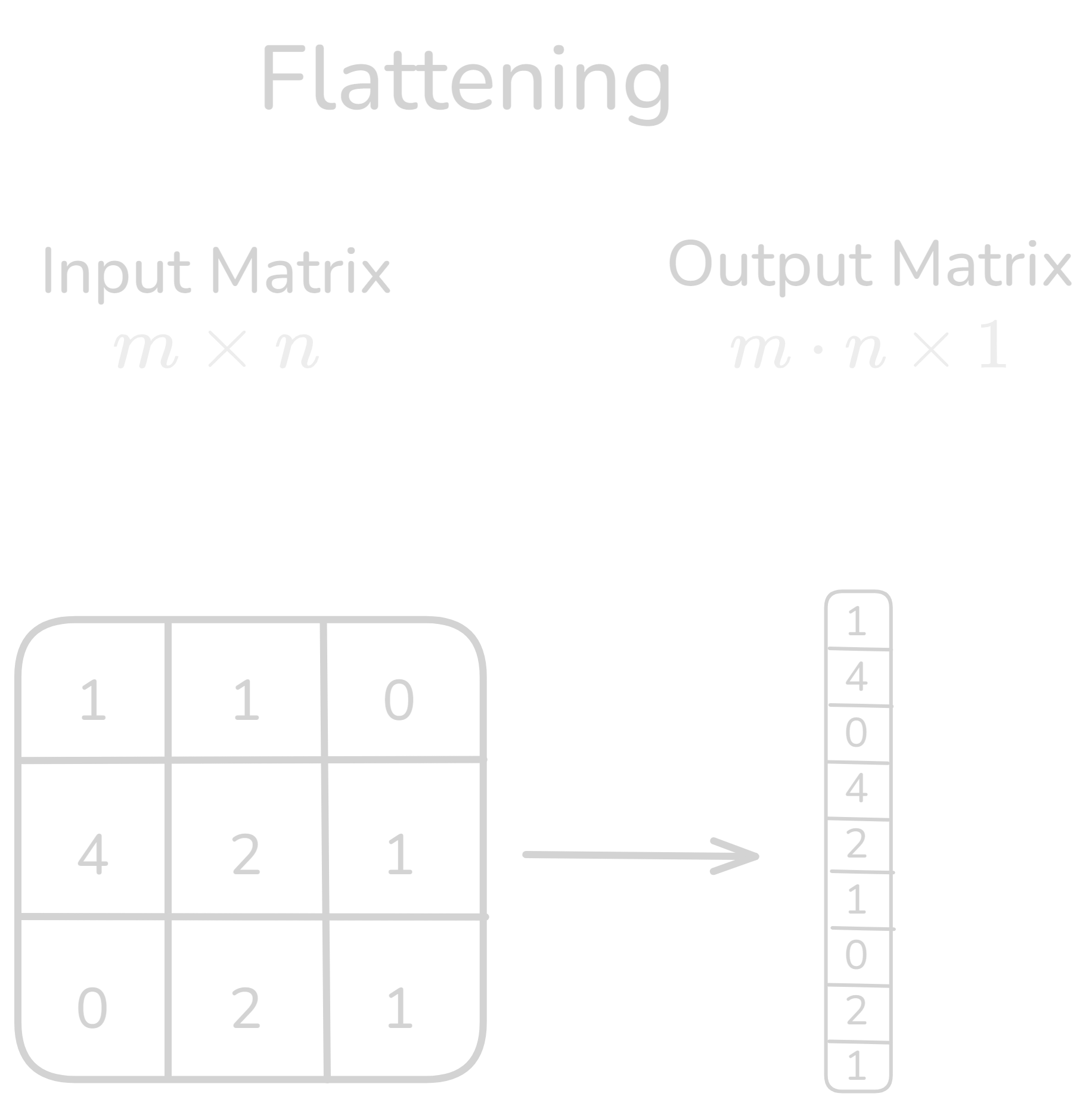 Figure 3.0: Flattening layer operation
Flattening in Convolutional Neural Networks (CNNs)
Definition: Flattening is a process in CNNs where the multi-dimensional output from the convolutional or pooling layers (typically 2D or 3D feature maps) is transformed into a one-dimensional vector. This vector can then be fed into fully connected layers (dense layers) for classification or regression tasks.
Flattening is essential because fully connected layers expect a one-dimensional input, but convolutional and pooling layers output multi-dimensional data. Flattening bridges this gap.
Formula :
Given an input tensor \(S\) of shape \((N, C, H, W)\), where:
- \(N\) is the batch size,
- \(C\) is the number of channels (or depth),
- \(H\) is the height of the feature map,
- \(W\) is the width of the feature map,
Flattening converts the tensor into a vector of size \((N, C \times H \times W)\). The general formula for flattening is simply:
\[f(S) = \text{reshape}(S, (N, C \times H \times W))\]The output is a one-dimensional vector that retains all the values from the original multi-dimensional array but without the spatial structure.
Use Case :
Feature Extraction: After convolution and pooling layers have extracted high-level features, flattening prepares the data for fully connected layers that perform the final classification.
Dimensionality Reduction: Although flattening does not reduce the total number of elements, it reduces the dimensions to a one-dimensional vector, suitable for input to classifiers.
Implementation with pytorch
1
2
3
4
5
6
7
8
9
# Example input tensor (batch size: 1, channels: 1, height: 4, width: 4)
input_tensor = torch.tensor([[[[1.0, 2.0, 3.0, 0.0],
                               [4.0, 5.0, 6.0, 1.0],
                               [3.0, 4.0, 7.0, 2.0],
                               [1.0, 2.0, 1.0, 0.0]]]])

# Flattening the input tensor
flatten_layer = nn.Flatten()
flattened_output = flatten_layer(input_tensor)
Other Operations in CNNs
Normalization Layer
Normalization layers are used to standardize input data by scaling them to a standard distribution. This helps improve the convergence of the network during training. One common type of normalization is Batch Normalization, which normalizes the output of the previous layer by adjusting and scaling the activations. It helps mitigate issues like internal covariate shift and improves model stability and performance.
ReLU (Rectified Linear Unit) Layer
The ReLU layer applies the activation function \(f(x) = \max(0, x)\), which introduces non-linearity into the model by zeroing out negative values. This makes it one of the most commonly used activation functions in CNNs.
Relu allows the model to learn complex patterns by introducing non-linear behavior, making it easier for the network to converge.
Softmax Layer
The softmax layer is typically used in the final output layer of a classification CNN. It converts the raw output scores into probabilities by exponentiating the values and normalizing them, ensuring that the output is a probability distribution over the classes.
Used for multi-class classification problems to output the probabilities for each class.
More on filters will be covered in subsequent posts.
Implementation
1
2
3
4
5
6
7
8
9
10
11
12
13
14
15
16
17
18
19
20
21
22
23
class ConvNet(nn.Module):
    def __init__(self, num_classes=10):
        super(ConvNet, self).__init__()
        self.layer1 = nn.Sequential(
            nn.Conv2d(1, 16, kernel_size=5, stride=1, padding=2),
            nn.BatchNorm2d(16),
            nn.ReLU(),
            nn.MaxPool2d(kernel_size=2, stride=2))
        self.layer2 = nn.Sequential(
            nn.Conv2d(16, 32, kernel_size=5, stride=1, padding=2),
            nn.BatchNorm2d(32),
            nn.ReLU(),
            nn.MaxPool2d(kernel_size=2, stride=2))
        self.fc = nn.Linear(7*7*32, num_classes)

    def forward(self, x):
        out = self.layer1(x)
        out = self.layer2(out)
        out = out.reshape(out.size(0), -1)
        out = self.fc(out)
        return out

model = ConvNet(num_classes).to(device)

Reference :
- https://en.wikipedia.org/wiki/Convolution
- https://en.wikipedia.org/wiki/Convolutional_neural_network
- https://readmedium.com/convolution-networks-for-dummies-aa8b086020ef