The 7 big time series fundamentals and operations
Introduction
Time series analysis evolved from early astronomical observations and economic studies in the 1920s. Box and Jenkins revolutionized the field in the 1970s with ARIMA models, while the Kalman filter (1960) transformed engineering and control systems. These foundational methods remain essential—even as neural networks dominate headlines. Whether you’re forecasting demand, modeling sensor data, or analyzing financial markets, these six concepts will sharpen your modeling decisions.
0. Heuristic Models (Baseline and Simple Methods)
Before jumping to complex models, master the foundational heuristic approaches that often serve as surprisingly strong baselines. These include naive forecasting, seasonal naive, moving averages, and exponential smoothing methods.
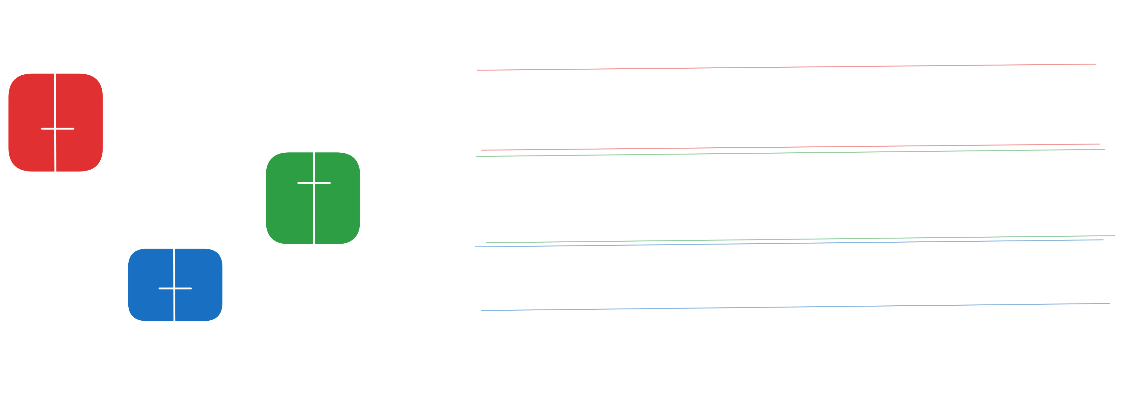
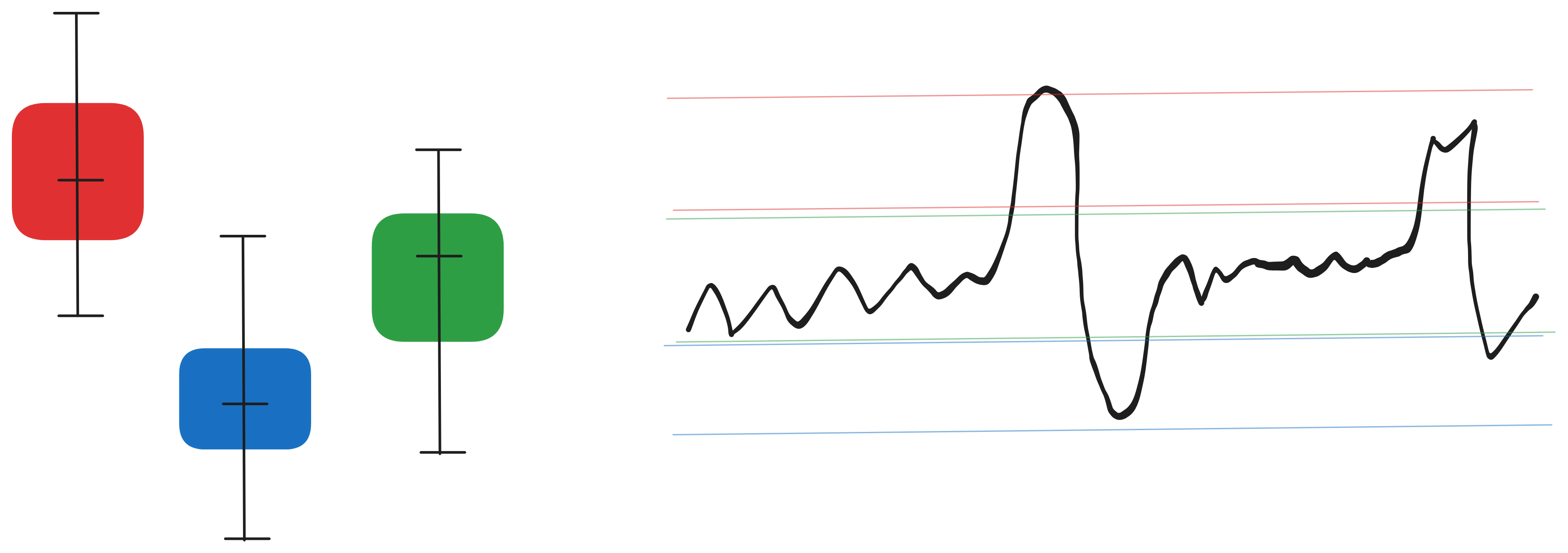 Figure 0.0: Boxplot-based group analysis (left) and time series with reference thresholds (right) for rule-based forecasting
Rule-Based (EDA-driven)
Start with the simplest setting: few discrete features and stable statistics. Using boxplots per group, test whether the median in group $g$ is stable across time. If stable, forecast that median. If recent means are more stable, use a moving mean. When seasonality dominates, repeat the seasonal lag value:
\[\hat{y}_t = \begin{cases} m_g & \text{if median stable} \\ \frac{1}{k}\sum_{i=1}^k y_{t-i} & \text{if recent mean stable} \\ y_{t-s} & \text{if seasonal lag robust} \\ y_{t-1} & \text{fallback} \end{cases}\]where $m_g = \mathrm{median}{y_j : j \in g}$.
This works well when group behavior is consistent, but fails when a new unseen group appears. This limitation pushes us toward stochastic models.
Naive Model
The simplest stochastic approach assumes the best forecast for tomorrow is today’s observation:
\[\hat{y}_{t+1} = y_t\]This works for random walks but fails with seasonality, where the error $e_{t+1}^{\text{Naive}} = (s_{t+1}-s_t)+(\epsilon_{t+1}-\epsilon_t)$ introduces bias.
Seasonal Naive
To handle seasonality, repeat the value from the same point in the previous season:
\[\hat{y}_{t+h} = y_{t+h-s}\]This removes seasonal bias but noise variance doubles: $\mathrm{Var}(e_{t+1}^{\text{SN}}) = 2\sigma^2$, making forecasts very noisy.
Moving Average
Smooth the noise by averaging the last $k$ points:
\[\hat{y}_{t+1} = \frac{1}{k}\sum_{i=0}^{k-1} y_{t-i}\]Noise variance drops to $\sigma^2/k$, but with a linear trend $y_t = a + bt + \epsilon_t$, you get bias: $b \cdot \frac{k+1}{2}$ because the average lags behind.
Tip: With seasonality, use seasonal smoothing (e.g., average each month across years) to avoid blurring the seasonal pattern.
Simple Exponential Smoothing (SES)
Assigns more weight to recent observations:
\[\hat{l}_t = \alpha y_t + (1 - \alpha) \hat{l}_{t-1},\] \[\hat{y}\_{t+1}^{\text{SES}} = \hat{l}\_t,\]where $0 < \alpha < 1$. Large $\alpha$ reacts quickly; small $\alpha$ smooths more. SES produces flat multi-step forecasts:
\[\hat{y}_{t+h}^{\text{SES}} = \hat{y}_{t+1},\]causing horizon-$h$ bias under a linear trend:
\[\mathbb{E}[\hat{y}_{t+h}^{\text{SES}} - y_{t+h}] \approx -b \left( h + \frac{1 - \alpha}{\alpha} \right),\]where $b$ is the trend slope.
Holt (Linear Trend)
Add a trend component $T_t$ alongside level $L_t$:
\[\begin{aligned} L_t &= \alpha y_t + (1-\alpha)(L_{t-1}+T_{t-1}) \\ T_t &= \beta(L_t-L_{t-1})+(1-\beta)T_{t-1} \\ \hat{y}_{t+h} &= L_t + hT_t \end{aligned}\]Now forecasts grow along slope $T_t$, eliminating trend bias. But seasonal effects remain in residuals.
Option: Use damped trend by multiplying $T_t$ by $\phi^h$ where $0<\phi<1$ when long-run growth shouldn’t explode.
Holt–Winters
Capture level, trend, and seasonality simultaneously. Additive version:
\[\begin{aligned} L_t &= \alpha(y_t - S_{t-s})+(1-\alpha)(L_{t-1}+T_{t-1}) \\ T_t &= \beta(L_t-L_{t-1})+(1-\beta)T_{t-1} \\ S_t &= \gamma(y_t-L_t)+(1-\gamma)S_{t-s} \\ \hat{y}_{t+h} &= L_t + hT_t + S_{t+h-s} \end{aligned}\]Multiplicative version: $\hat{y}{t+h} = (L_t + hT_t)\times S{t+h-s}$. Choose additive when seasonal amplitude is constant; multiplicative when it grows with the level. Understanding these simple methods teaches you about the fundamental components of time series and provides benchmarks that sophisticated models must beat.
⚠️ Important Note
These heuristic methods are not just academic exercises—they often outperform complex ML models in practice, especially with limited data (<100 observations) or stable patterns. Always benchmark against them. They’re also:
- Fast: Real-time forecasting with minimal compute
- Interpretable: Each parameter has clear meaning ($\alpha$ = responsiveness, $s$ = season length)
- Robust: Less prone to overfitting than models with many parameters
When they fail
- Multiple seasonal patterns (daily + weekly + yearly)
- External regressors needed (promotions, holidays, weather)
- Structural breaks or regime changes
- Non-stationary variance requiring transformations beyond log/sqrt
Validation
Never use random train/test splits—use time-ordered splits or expanding window CV. A model that “predicts the past” using future information is worthless. Test on out-of-sample horizons matching your actual forecasting task.
1. Stationarity and Non-Stationarity
A stationary series has constant mean, variance, and autocovariance over time. Most forecasting methods assume stationarity, making it crucial to master differencing, detrending, and transformation techniques.
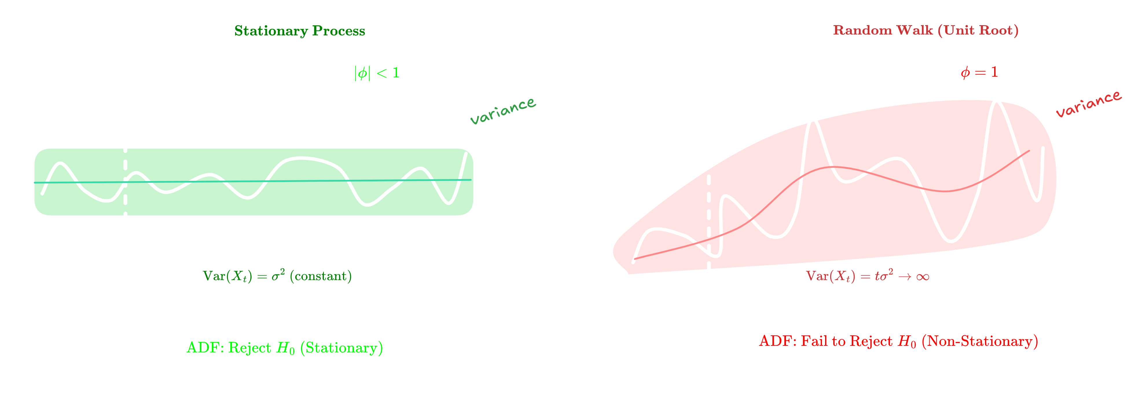
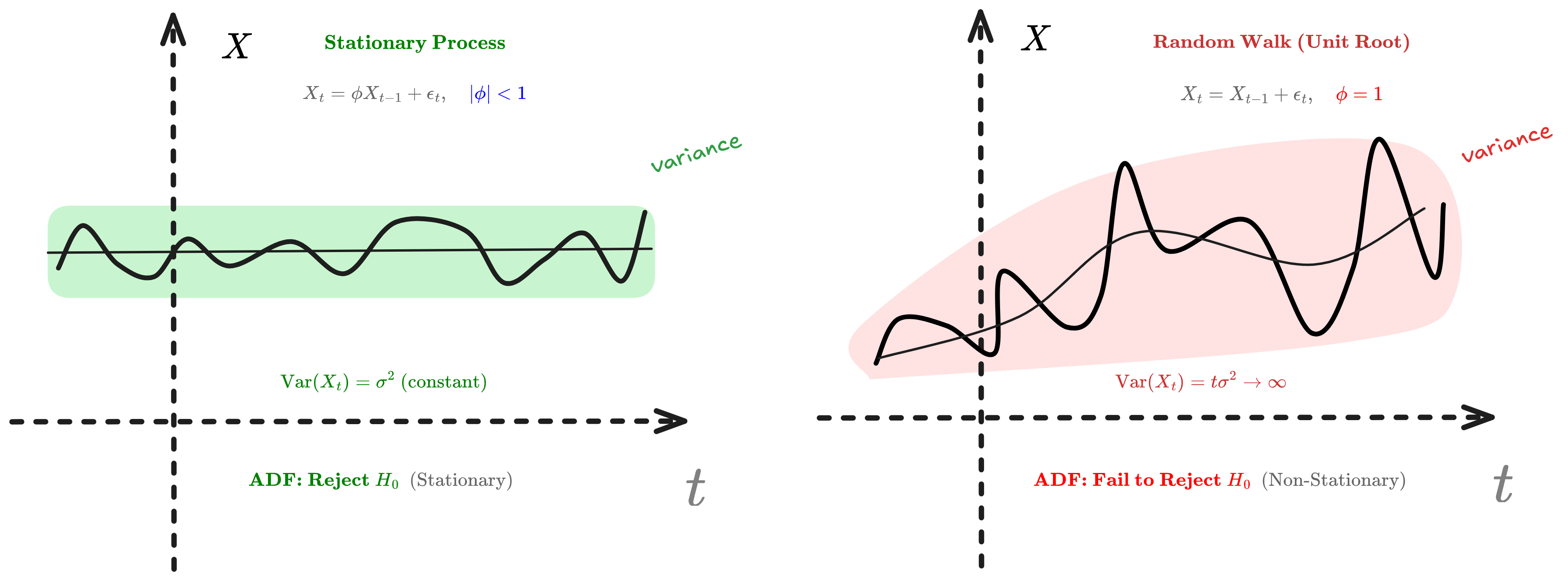 Figure 1.0 : Random walk vs Stationnary series Illustration
Weak Stationarity
Weak stationarity requires:
- $E[X_t] = \mu$ for all $t$ (constant mean)
- $\text{Var}(X_t) = \sigma^2$ for all $t$ (constant variance)
- $\text{Cov}(X_t, X_{t+h}) = \gamma(h)$ depends only on lag $h$, not on $t$
Consider the random walk $X_t = X_{t-1} + \epsilon_t$ where $\epsilon_t \sim \text{WN}(0, \sigma^2)$. The variance grows unbounded: $\text{Var}(X_t) = t\sigma^2 \to \infty$, proving non-stationarity.
However, the first difference $\nabla X_t = X_t - X_{t-1} = \epsilon_t$ is stationary. This demonstrates why differencing works: it transforms integrated processes $I(d)$ into stationary ones.
The ADF test checks whether $\phi = 1$ in $X_t = \phi X_{t-1} + \epsilon_t$.
If $|\phi| < 1$, the process is mean-reverting (stationary). If $\phi = 1$, it exhibits a unit root (random walk).
The test statistic follows a non-standard Dickey-Fuller distribution because under the null hypothesis, the process is non-stationary.
Key insight: Always test for stationarity before modeling. If non-stationary, apply differencing or transformations until you achieve stationarity.
2. Autocorrelation and Partial Autocorrelation
What is Autocorrelation?
Autocorrelation (serial correlation) quantifies the linear relationship between a time series and a lagged version of itself. It measures temporal dependence—the degree to which past values inform future values.
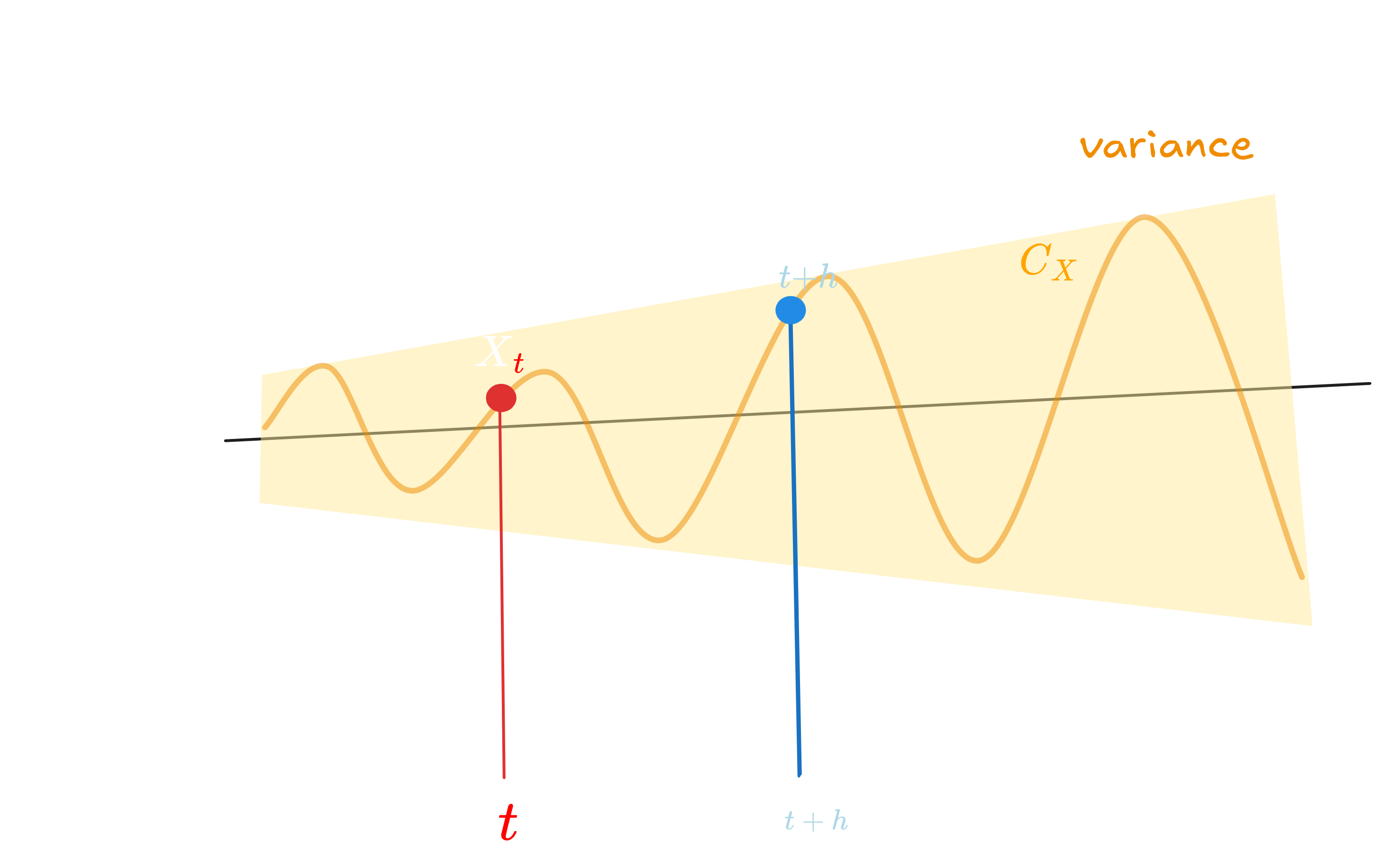
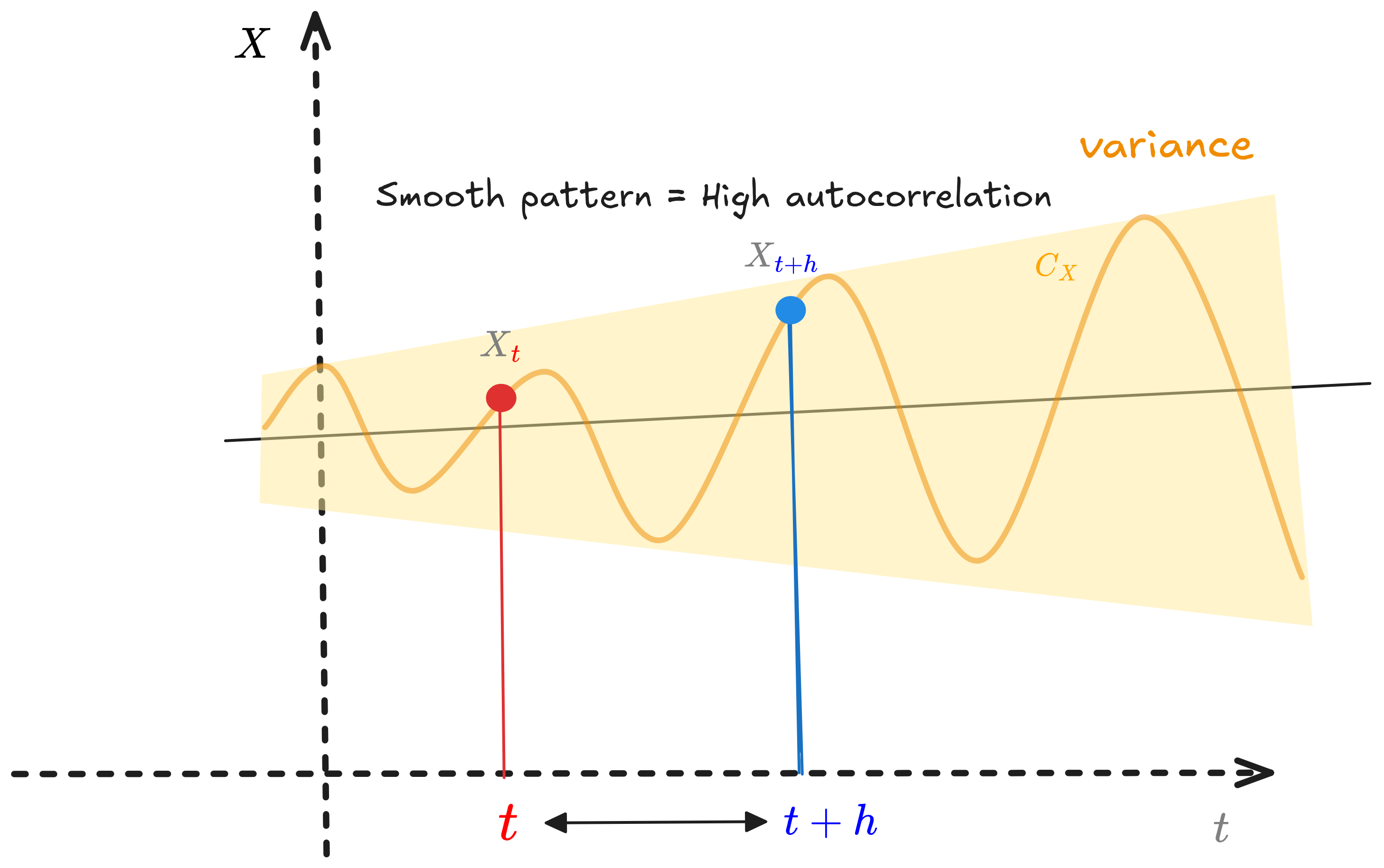 Figure 2.0 : Simple Autocorrelation Illustration
Autocorrelation at lag $h$
\[\rho(h) = \frac{\gamma(h)}{\gamma(0)} = \frac{\text{Cov}(X_t, X_{t+h})}{\text{Var}(X_t)} = \frac{E[(X_t - \mu)(X_{t+h} - \mu)]}{\sigma^2}\]Properties:
- $\rho(0) = 1$ (perfect self-correlation)
- $-1 \leq \rho(h) \leq 1$ (bounded by correlation coefficient limits)
- $\rho(h) = \rho(-h)$ (symmetric in stationary processes)
High autocorrelation $\lvert\rho(h)\rvert \approx 1$ indicates strong temporal dependence with smooth, predictable patterns.
Low autocorrelation $\lvert\rho(h)\rvert \approx 0$ suggests independence, approaching white noise where forecasting is impossible.
Understanding Lags
A lag is a temporal displacement operator. For a time series ${X_1, X_2, \ldots, X_T}$, the lag-$h$ operator $L^h$ yields $L^h X_t = X_{t-h}$.
Informative lags
Informative lags satisfy these criteria:
Statistical significance: The autocorrelation $\hat{\rho}(h)$ exceeds the $95\%$ confidence bounds $\pm 1.96/\sqrt{T}$, indicating correlation beyond random chance.
Domain alignment: Lags correspond to known periodicities—lag 7 for daily data with weekly patterns, lag 12 for monthly data with annual seasonality, lag 24 for hourly data with daily cycles.
Causal plausibility: The relationship has mechanistic justification—yesterday’s temperature influences today’s through atmospheric inertia, last quarter’s sales inform current planning.
Parsimony: Including lags beyond those capturing essential dynamics risks overfitting. Balance explanatory power against model complexity.
Uninformative lags
Uninformative lags exhibit:
Statistical insignificance ($ \hat{\rho}(h) < 1.96/\sqrt{T}$) - Spurious correlations from non-stationarity
- Computational burden without predictive gain
- Data insufficiency (lag $h$ requires at least $T - h$ observations; keep $h < T/10$)
ACF vs PACF: The Key Difference
These concepts reveal temporal dependencies in your data. The ACF (Autocorrelation Function) shows correlation between a value and its lags, while PACF (Partial Autocorrelation Function) shows the direct relationship after removing indirect effects.
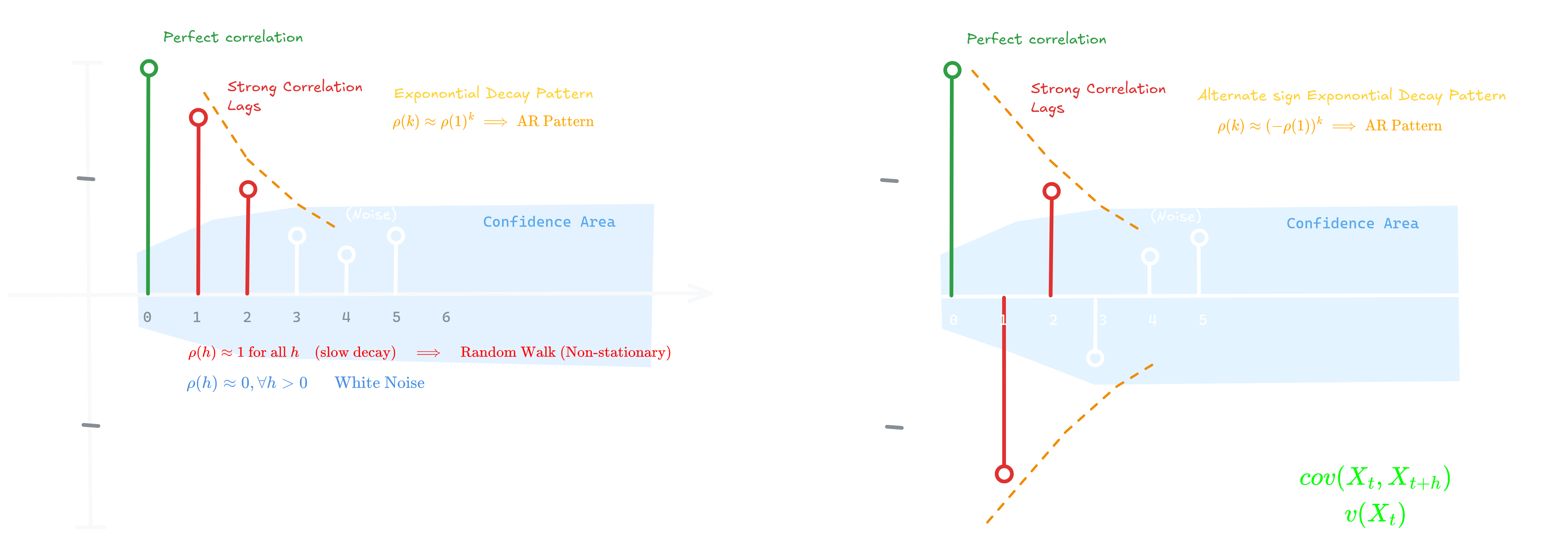
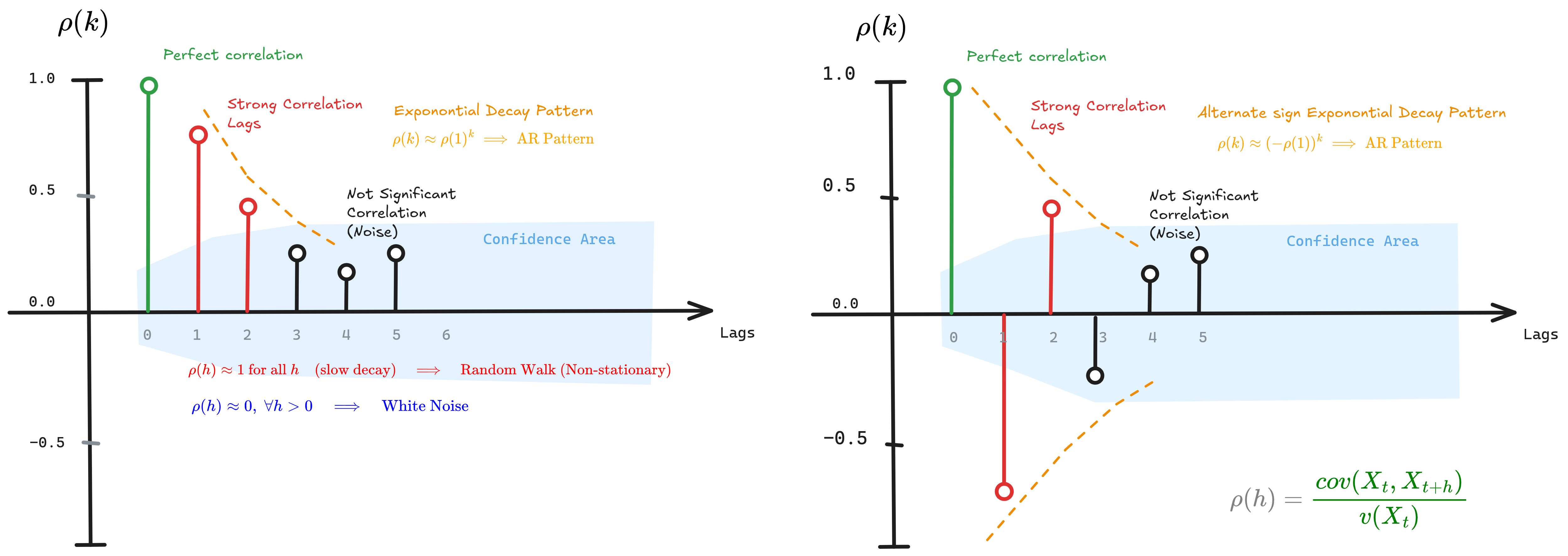 Figure 2.1: ACF plots showing exponential decay patterns, confidence bounds, and interpretation for AR processes, random walks, and white noise
Autocorrelation Function
\[\rho(h) = \frac{\gamma(h)}{\gamma(0)} = \frac{\text{Cov}(X_t, X_{t+h})}{\text{Var}(X_t)}\]where $\gamma(h) = \text{Cov}(X_t, X_{t+h})$ is the autocovariance at lag $h$, and $\gamma(0) = \text{Var}(X_t)$ normalizes the measure to the range $[-1, 1]$.
Partial Autocorrelation Function
Partial autocorrelation $\phi_{hh}$ measures correlation between $X_t$ and $X_{t+h}$ after removing the linear dependence on intermediate lags $X_{t+1}, \ldots, X_{t+h-1}$. This isolates the unique, direct contribution of lag $h$ beyond what’s already explained by shorter lags.
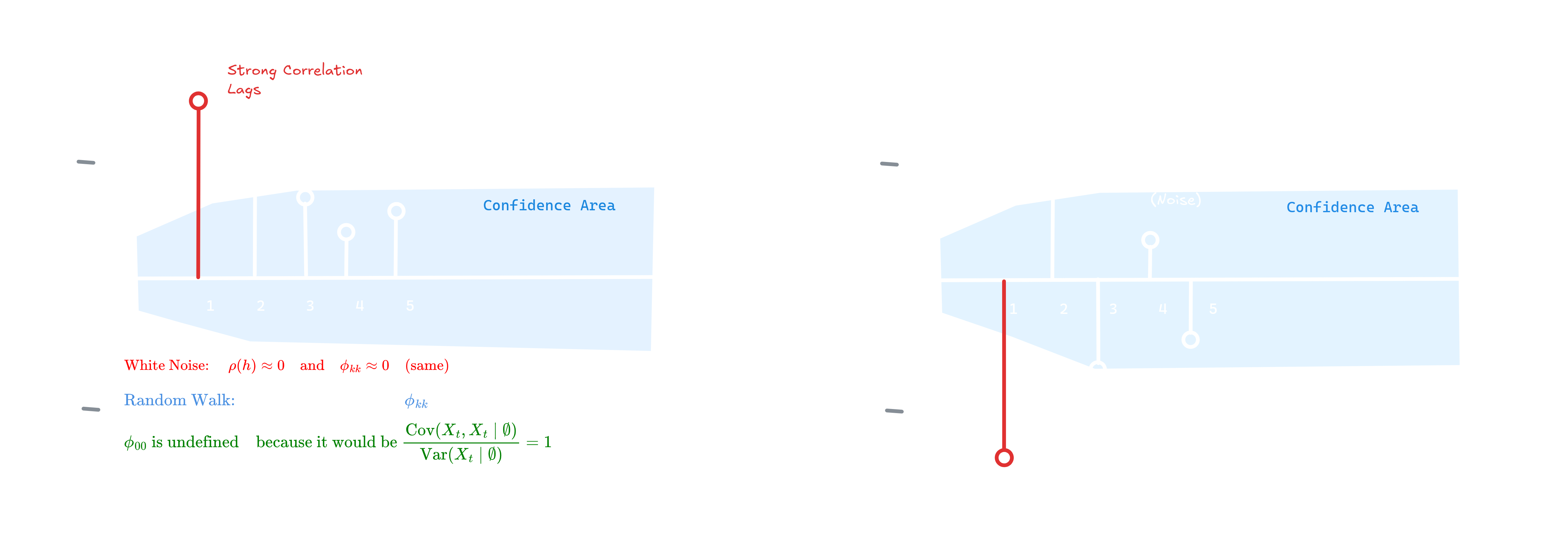
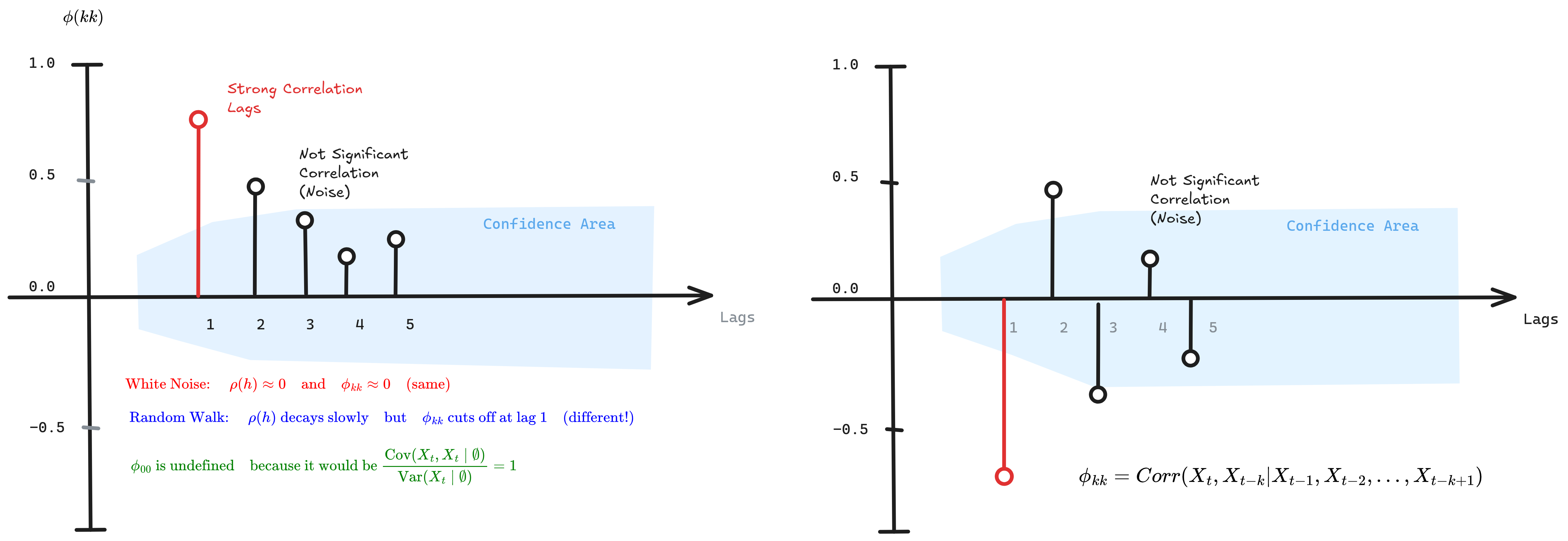 Figure 2.2: PACF plots showing sharp cutoffs for AR processes, with comparison between white noise and random walk behavior
Pattern Recognition: Model Selection Guide
For AR(p) processes, the PACF cuts off sharply after lag $p$ (i.e., $\phi_{hh} = 0$ for $h > p$), while the ACF decays exponentially or shows damped sinusoids. For MA(q) processes, the pattern inverts: ACF cuts off after lag $q$, while PACF decays gradually. This duality enables visual identification of model order.
| ACF Pattern | PACF Pattern | Process Type | Identification Rule |
|---|---|---|---|
| Exponential decay | Sharp cutoff at lag p | AR(p) | Count significant PACF lags |
| Sharp cutoff at lag q | Exponential decay | MA(q) | Count significant ACF lags |
| Gradual decay | Gradual decay | ARMA(p,q) | Use information criteria (AIC/BIC) |
| Very slow decay | Spike at lag 1, then small | Non-stationary | Apply differencing: $\nabla X_t = X_t - X_{t-1}$ |
| All within bounds | All within bounds | White noise | No predictable structure |
Why these patterns emerge
AR(p) Process
\[X_t = \phi_1 X_{t-1} + \phi_2 X_{t-2} + \cdots + \phi_p X_{t-p} + \varepsilon_t\]The Yule-Walker equations describe the recursive structure:
\[\rho(h) = \phi_1 \rho(h-1) + \phi_2 \rho(h-2) + \cdots + \phi_p \rho(h-p)\]This recursion creates infinite memory through exponential decay in the ACF. However, only the first $p$ lags have direct effects on $X_t$, causing the PACF to vanish for $h > p$.
MA(q) Process
\[X_t = \varepsilon_t + \theta_1 \varepsilon_{t-1} + \theta_2 \varepsilon_{t-2} + \cdots + \theta_q \varepsilon_{t-q}\]MA processes have finite memory—exactly $q$ periods. Beyond lag $q$, $X_t$ and $X_{t+h}$ share no common shock terms, yielding $\rho(h) = 0$ for $h > q$. The PACF decays because expressing this finite-memory relationship without intermediate values requires a complex infinite representation.
Practical tip: Plot both ACF and PACF before choosing your model. The cutoff patterns immediately suggest whether you need AR terms, MA terms, or both (ARMA). Non-stationarity shows as persistent high ACF values—difference the series until the ACF decays rapidly.
The Double-Edged Sword
When Autocorrelation Weakens: Classification
Standard supervised learning algorithms assume independent, identically distributed (i.i.d.) observations. Temporal dependence violates this assumption, creating several pathologies:
1. Effective sample size reduction: Correlated observations provide less information than independent ones. The effective degrees of freedom $T_{\text{eff}} < T$ deflates statistical power.
2. Inflated Type I error rates: Standard errors underestimate true variability, yielding spuriously significant results and overconfident predictions.
3. Information leakage in cross-validation: Random k-fold splitting places temporally adjacent observations in training and test sets, allowing models to exploit short-term autocorrelation that won’t generalize to future data.
4. Overfitting to temporal structure: Classifiers learn “if previous observation was class A, current observation is class A” rather than discriminative features, failing when temporal patterns shift.
Remediation strategies
Time series cross-validation: Strictly respect temporal ordering—train on $t \in [1, T_{\text{train}}]$, validate on $t \in [T_{\text{train}} + \text{gap}, T_{\text{test}}]$. The gap prevents leakage from short-term autocorrelation.
Differencing transformation: Apply $\nabla X_t = X_t - X_{t-1}$ or $\nabla_s X_t = X_t - X_{t-s}$ (seasonal) to remove autocorrelation structure. Verify via Ljung-Box test.
Specialized algorithms: ROCKET (random convolutional kernels), InceptionTime (deep inception networks), and BOSS (bag of symbolic patterns) are designed to handle temporal dependence while maintaining discriminative power.
When Autocorrelation Strengthens: Forecasting
Temporal dependence is the foundation of predictability. Without autocorrelation, time series reduces to white noise—inherently unforecastable.
1. Lagged predictors: Past values $X_{t-1}, X_{t-2}, \ldots, X_{t-p}$ become features. The autoregressive structure $X_t = f(X_{t-1}, \ldots, X_{t-p})$ directly exploits autocorrelation.
2. Model specification guidance: ACF/PACF patterns reveal optimal model orders:
- Significant PACF at lags $1, \ldots, p$ → AR(p)
- Significant ACF at lags $1, \ldots, q$ → MA(q)
- Both decay → ARMA(p,q)
3. Efficiency gains: Properly specified models that capture autocorrelation structure minimize forecast error variance. Ignoring autocorrelation leaves predictable patterns in residuals, sacrificing accuracy.
4. Temporal aggregation: Strong autocorrelation enables aggregation—forecasting the sum $\sum_{t=1}^{h} X_t$ often has lower relative error than individual forecasts due to error cancellation.
Optimal practices
- Include domain-informed lags (lag-7 for weekly patterns, lag-12 for annual seasonality in monthly data)
- Model autocorrelation explicitly (ARIMA, SARIMA, VAR)
- For complex dependencies, employ recurrent architectures (LSTM, GRU) that maintain hidden state across time steps
Essential Statistical Tests
1. Ljung-Box Test
Null hypothesis: $H_0: \rho(1) = \rho(2) = \cdots = \rho(h) = 0$ (white noise)
Test statistic:
\[Q_{\text{LB}} = T(T+2) \sum_{k=1}^{h} \frac{\hat{\rho}^2(k)}{T-k} \sim \chi^2(h)\]where $T$ is sample size and $h$ is the maximum lag tested. Rejection of $H_0$ (p-value $< 0.05$) indicates significant autocorrelation structure.
Application: Diagnostic for model residuals—properly specified models should yield white noise errors. Also used to test whether differencing or detrending successfully removed autocorrelation.
1
2
3
4
from statsmodels.stats.diagnostic import acorr_ljungbox

result = acorr_ljungbox(residuals, lags=10)
# p-value < 0.05 → autocorrelation remains (model misspecification)
2. Augmented Dickey-Fuller (ADF) Test
Null hypothesis: $H_0$: Unit root present (non-stationary)
Test equation:
\[\Delta X_t = \alpha + \beta t + \gamma X_{t-1} + \sum_{i=1}^{p}\delta_i \Delta X_{t-i} + \varepsilon_t\]Tests whether $\gamma = 0$ (unit root) versus $\gamma < 0$ (stationary around trend). Augmentation terms $\Delta X_{t-i}$ control for serial correlation.
Interpretation:
- p-value $< 0.05$: Reject $H_0$ → series is stationary
- p-value $> 0.05$: Fail to reject → series is non-stationary, apply differencing
Critical: Non-stationary series exhibit spurious correlations and invalidate standard time series models. Always test before modeling.
1
2
3
4
5
from statsmodels.tsa.stattools import adfuller

adf_stat, p_value = adfuller(series)[:2]
if p_value > 0.05:
    series = np.diff(series)  # First differencing
3. Durbin-Watson Test
Tests: First-order autocorrelation in regression residuals
\[\text{DW} = \frac{\sum_{t=2}^{T}(e_t - e_{t-1})^2}{\sum_{t=1}^{T}e_t^2} \approx 2(1 - \hat{\rho}(1))\]Decision rule:
- $\text{DW} \approx 2$: No first-order autocorrelation ($\hat{\rho}(1) \approx 0$)
- $\text{DW} < 2$: Positive autocorrelation (successive errors move together)
- $\text{DW} > 2$: Negative autocorrelation (successive errors alternate)
Limitation: Only detects lag-1 autocorrelation; use Ljung-Box or Breusch-Godfrey for higher orders.
1
2
3
4
from statsmodels.stats.stattools import durbin_watson

dw = durbin_watson(model.resid)
# Ideal: 1.5 < DW < 2.5
3. State Space Models and Kalman Filtering
State space models separate observed measurements from underlying hidden states, allowing you to model complex dynamics while accounting for measurement noise and uncertainty.
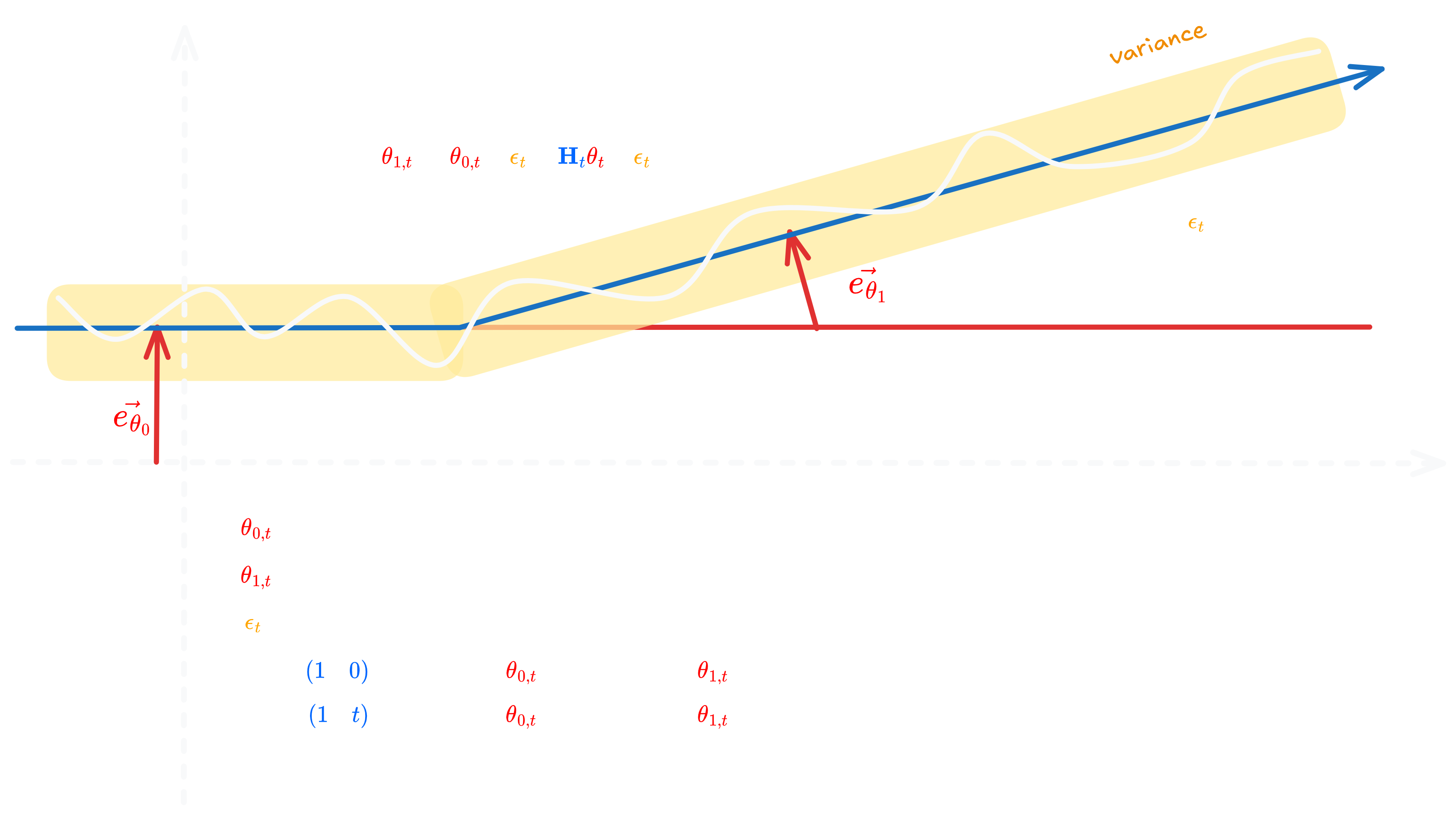
 Figure 3.0: State space representation showing level and slope components with observation noise, illustrating the Local Linear Trend Model
The general form consists of two equations:
State equation:
\[\theta_t = F_t \theta_{t-1} + G_t \eta_t, \quad \eta_t \sim \mathcal{N}(0, Q_t)\]Observation equation:
\[X_t = H_t \theta_t + \epsilon_t, \quad \epsilon_t \sim \mathcal{N}(0, R_t)\]Process noise $\eta_t$ allows hidden states to evolve unpredictably, capturing real-world randomness. Measurement noise $\epsilon_t$ accounts for imperfect observations. Both are assumed independent and normally distributed.
The Kalman Filter
The Kalman Filter recursively estimates the state and its uncertainty through prediction and update steps:
Prediction:
\[\begin{aligned} \theta_{t|t-1} &= F_t \theta_{t-1|t-1} \\ P_{t|t-1} &= F_t P_{t-1|t-1} F_t^T + G_t Q_t G_t^T \end{aligned}\]Update:
\[\begin{aligned} K_t &= P_{t|t-1} H_t^T (H_t P_{t|t-1} H_t^T + R_t)^{-1} \\ \theta_{t|t} &= \theta_{t|t-1} + K_t(X_t - H_t \theta_{t|t-1}) \\ P_{t|t} &= (I - K_t H_t) P_{t|t-1} \end{aligned}\]The Kalman gain $K_t$ determines how much to adjust the state estimate based on the innovation \(X_t - H_t \theta_{t|t-1}\) (the “surprise” in the new observation). For linear Gaussian models, the filter is optimal—it minimizes mean squared error.
Why it matters: State space models unify many time series approaches and excel at handling missing data, real-time forecasting, and signal extraction. They form the basis for particle filters and sequential Monte Carlo methods.
Example
Setup: Track an object with hidden state $\theta_t = \begin{bmatrix} p_t \ v_t \end{bmatrix}$, observing only noisy position.
Matrices:
\[F = \begin{bmatrix} 1 & 1 \\ 0 & 1 \end{bmatrix}, \quad H = \begin{bmatrix} 1 & 0 \end{bmatrix}, \quad Q = \begin{bmatrix} 0.1 & 0 \\ 0 & 0.1 \end{bmatrix}, \quad R = 2\]Initial:
\[\theta_{0|0} = \begin{bmatrix} 0 \\ 5 \end{bmatrix}, \quad P_{0|0} = I_2\]Prediction:
\[\begin{aligned} \theta_{1|0} &= F \theta_{0|0} = \begin{bmatrix} 5 \\ 5 \end{bmatrix} \\ P_{1|0} &= F P_{0|0} F^T + Q = \begin{bmatrix} 2.1 & 1 \\ 1 & 1.1 \end{bmatrix} \end{aligned}\]Update (observation $X_1 = 4.8$):
\[\begin{aligned} K_1 &= \begin{bmatrix} 0.51 \\ 0.24 \end{bmatrix} \\ \theta_{1|1} &= \begin{bmatrix} 5 \\ 5 \end{bmatrix} + \begin{bmatrix} 0.51 \\ 0.24 \end{bmatrix}(4.8 - 5) = \begin{bmatrix} 4.90 \\ 4.95 \end{bmatrix} \end{aligned}\]Interpretation: Predicted position = 5, observed 4.8. The filter corrects both position and velocity using the Kalman gain, which balances prediction uncertainty against measurement noise.
4. Spectral Analysis and Frequency Domain Methods
While most work happens in the time domain, spectral analysis transforms data into the frequency domain using Fourier transforms and periodograms. This reveals cyclical patterns, seasonal components, and hidden periodicities that are difficult to detect in raw time series.
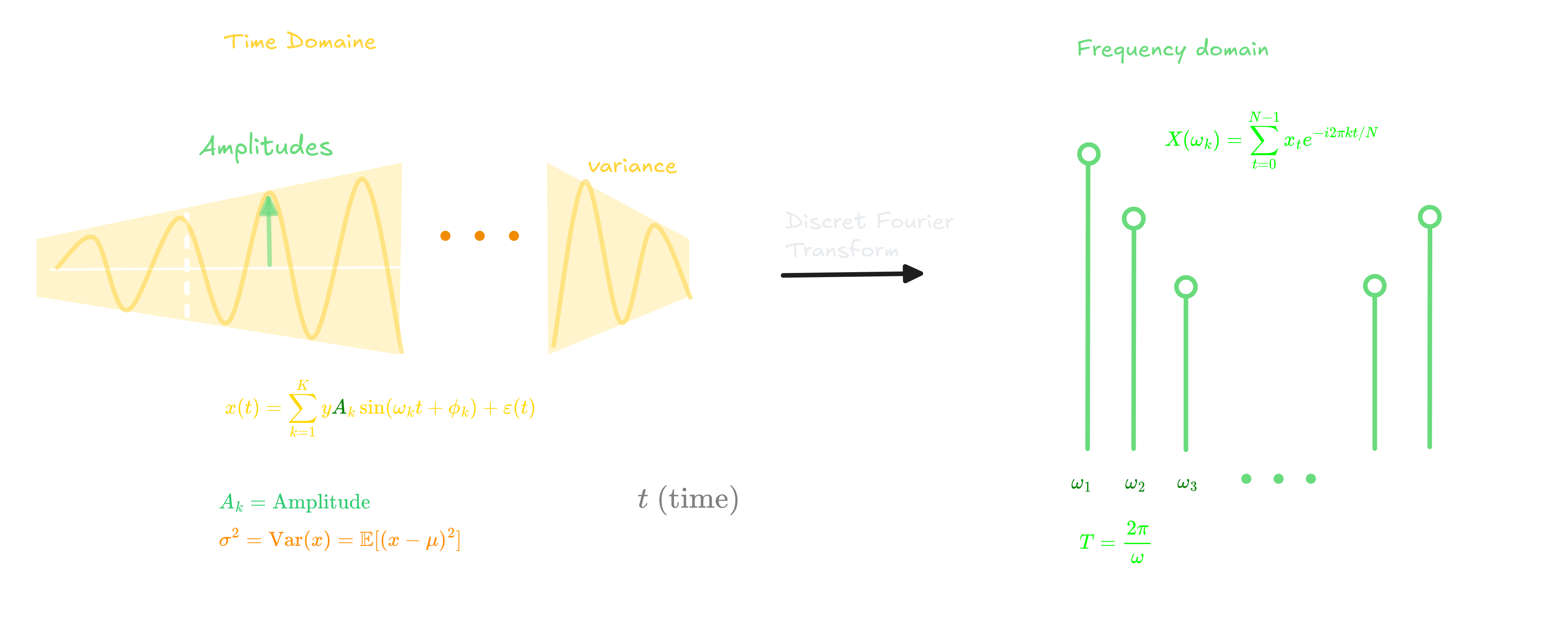
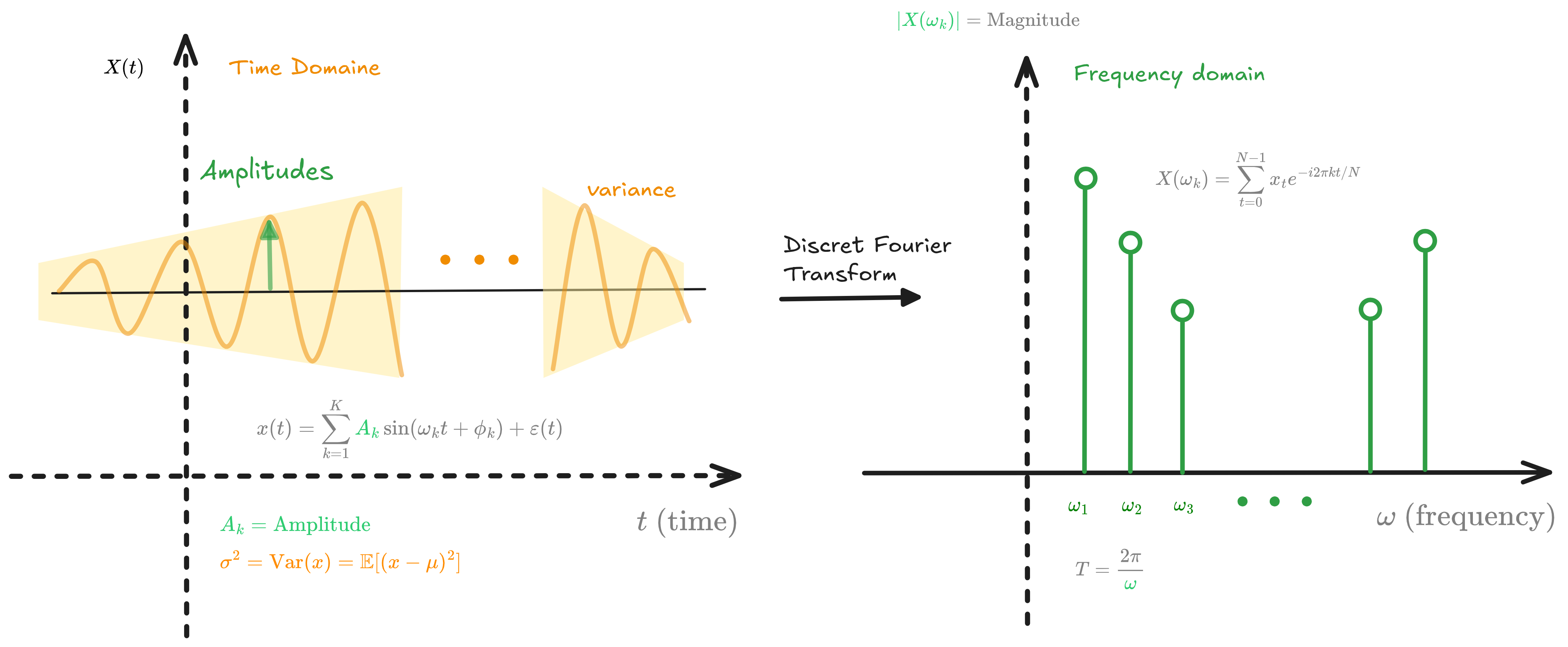 Figure 4.0: Time domain to frequency domain transformation via DFT, showing how sinusoidal components map to frequency magnitudes
Discrete Fourier Transform
The Discrete Fourier Transform (DFT) decomposes a time series into sinusoidal components:
\[X(\omega_k) = \sum_{t=0}^{N-1} x_t e^{-i2\pi k t/N}, \quad k = 0, 1, \ldots, N-1\]where $\omega_k = 2\pi k/N$ is the frequency and $i = \sqrt{-1}$. Each frequency $\omega_k$ reveals how much a particular cycle contributes to the overall signal.
Periodogram
The periodogram estimates the power spectral density:
\[I(\omega_k) = \frac{1}{N}\left|X(\omega_k)\right|^2 = \frac{1}{N}\left|\sum_{t=0}^{N-1} x_t e^{-i2\pi k t/N}\right|^2\]This shows how variance is distributed across frequencies. Peaks in the periodogram identify dominant cycles—a peak at frequency $\omega$ indicates a cycle with period $T = 2\pi/\omega$.
Spectral Density
For stationary processes, the spectral density $S(\omega)$ relates to the autocovariance function $\gamma(h)$ through:
\[S(\omega) = \sum_{h=-\infty}^{\infty} \gamma(h) e^{-i\omega h}\]This is the Fourier transform of the ACF, showing that time domain (autocorrelation) and frequency domain (spectral density) are equivalent representations.
Wavelet Transforms
Wavelet transforms extend Fourier analysis to non-stationary signals by using localized basis functions:
\[W(a,b) = \int_{-\infty}^{\infty} x(t) \psi^*\left(\frac{t-b}{a}\right) dt\]where $\psi$ is the mother wavelet, $a$ is the scale (inversely related to frequency), $b$ is the position in time, and $*$ denotes complex conjugate. This allows you to see how frequency content changes over time—essential for signals with evolving dynamics.
Wavelet Transform Properties
The wavelet transform defines a smooth, invertible mapping from the time domain to the time-scale (wavelet) domain.
Mathematically, this is an isometric embedding:
\[\mathcal{W}: L^2(\mathbb{R}) \hookrightarrow L^2(\mathbb{R}^+ \times \mathbb{R}, \frac{da,db}{a^2})\]that preserves energy and admits a well-defined inverse. The transformation is smooth in the sense that if $x(t)$ is continuous or differentiable, so are the wavelet coefficients $W(a,b)$ as functions of $a$ and $b$.
While not strictly bijective (it maps a 1D signal to a 2D representation), the transform is invertible through the reconstruction formula:
\[x(t) = \frac{1}{C_\psi} \iint W(a,b) \psi_{a,b}(t) \, \frac{da \, db}{a^2}\]where $C_\psi$ is the admissibility constant. This inverse exists whenever the mother wavelet satisfies the admissibility condition, ensuring perfect reconstruction.
The ensemble of basis functions ${\psi_{a,b}(t) = \frac{1}{\sqrt{a}} \psi(\frac{t-b}{a})}$ forms a continuous frame that spans the signal space, providing a redundant but stable representation.
Wavelet Gradient
The gradient of the wavelet transform provides crucial information about how wavelet coefficients change across the time-frequency plane:
\[\nabla W(a,b) = \left(\frac{\partial W}{\partial a}, \frac{\partial W}{\partial b}\right)\]This gradient captures two essential dynamics:
- $\frac{\partial W}{\partial a}$ reveals how energy concentration changes across scales (frequencies)
- $\frac{\partial W}{\partial b}$ shows temporal evolution of spectral content
The gradient magnitude $|\nabla W|$ identifies ridges in the scalogram—curves of maximum energy concentration that trace evolving frequency components over time. These ridges are particularly valuable for extracting instantaneous frequency trajectories in non-stationary signals, enabling precise characterization of chirps, glissandos, and other time-varying phenomena.
Benefits of the Gradient Formulation
The gradient $\nabla W = (\frac{\partial W}{\partial a}, \frac{\partial W}{\partial b})$ enables:
- Ridge detection for extracting dominant time-frequency structures
- Edge sharpening for improved segmentation and anomaly detection
- Adaptive denoising through gradient-guided thresholding
- Multiresolution edge detection capturing both fine and coarse features
- Synchrosqueezing transforms that sharpen time-frequency representations by reassigning coefficients along gradient directions—particularly valuable in speech processing, biomedical signal analysis, and gravitational wave detection
Mother Wavelets
The wavelet transform can be understood as an inner product $W \propto \langle x, \psi_{a,b} \rangle$, measuring how similar the signal is to the scaled and shifted wavelet at each point. The mother wavelet $\psi(t)$ serves as the basis function.
Common choices include:
- Morlet wavelet: $\psi(t) = e^{i\omega_0 t}e^{-t^2/2}$, which provides excellent time-frequency localization
- Mexican Hat wavelet: for edge detection
- Haar wavelet: for discrete decomposition
Energy and Scalogram
The energy of the wavelet decomposition is given by:
\[E = \iint |W(a,b)|^2 \, da \, db\]This represents the total signal energy distributed across all scales and time positions. The wavelet scalogram visualizes $|W(a,b)|^2$ as a heatmap, with color intensity showing energy concentration.
Uncertainty Principle
An important property of wavelets is the uncertainty principle:
\[\Delta t \cdot \Delta f \geq \frac{1}{4\pi}\]This establishes a fundamental limit on simultaneous time and frequency resolution. Unlike the Short-Time Fourier Transform (STFT) with fixed resolution, wavelets provide adaptive resolution:
- High temporal resolution at high frequencies (small $a$) to capture rapid changes
- High frequency resolution at low frequencies (large $a$) to identify long-term trends
When to Use Spectral Methods
Spectral methods excel when your data has complex cyclical structures:
- Think economic cycles, biological rhythms, or signal processing applications
- Use Fourier for stationary periodic patterns
- Use wavelets when frequency content varies over time, such as:
- Seismic signals
- Speech analysis
- Financial time series with regime changes
- Any signal with transient events and non-stationary characteristics
The gradient formulation is particularly powerful for applications requiring precise feature localization:
- Detecting epileptic seizures in EEG data
- Analyzing gravitational waves
- Tracking vocal formants in speech processing
5. Multivariate Time Series and Causality
Move beyond univariate analysis to understand relationships between multiple time series. Vector Autoregression (VAR) models systems of equations where each variable depends on its own lags and the lags of other variables. Cointegration captures long-run equilibrium relationships between non-stationary series that move together over time.
Granger causality tests whether one time series helps predict another beyond what the target series’ own history provides. This doesn’t prove true causation, but identifies predictive relationships that inform modeling decisions.
Critical for: Economic modeling, financial systems, sensor networks, and any domain where multiple interacting processes evolve together. Understanding these relationships often matters more than predicting any single series accurately.
6. Ergodicity, Ensemble vs Time Averages, and Non-Ergodic Processes
Ergodicity means time averages equal ensemble averages—studying one realization over time gives you the same information as studying many realizations at one point. Most statistical methods assume ergodicity, but many real-world processes are non-ergodic.
In non-ergodic systems (financial markets, evolutionary processes, path-dependent phenomena), past observations may not represent future possibilities. Individual trajectories diverge dramatically, and the concept of a stable “true” parameter becomes questionable.
This fundamentally changes forecasting: traditional methods assume the future resembles the past statistically. In non-ergodic systems, this breaks down. You need robust decision-making frameworks rather than point forecasts.
Why it matters: Understanding ergodicity helps you recognize when traditional forecasting fails, why backtesting can be misleading, and when you should focus on risk management instead of prediction. This concept bridges statistics, physics, and philosophy—fundamentally changing how you think about uncertainty.